<?xml version="1.0" encoding="utf-8"?><feed xmlns="http://www.w3.org/2005/Atom" ><generator uri="https://jekyllrb.com/" version="3.10.0">Jekyll</generator><link href="https://abeljansma.nl/feed.xml" rel="self" type="application/atom+xml" /><link href="https://abeljansma.nl/" rel="alternate" type="text/html" /><updated>2026-05-21T08:35:20+00:00</updated><id>https://abeljansma.nl/feed.xml</id><title type="html">Abel Jansma</title><subtitle>Abel Jansma is a scientist studying emergence, higher-order interactions, information theory, and complex systems across biology and artificial intelligence.</subtitle><author><name>Abel Jansma</name></author><entry><title type="html">A short koan about the spider Oza</title><link href="https://abeljansma.nl/2025/10/28/ozakoan.html" rel="alternate" type="text/html" title="A short koan about the spider Oza" /><published>2025-10-28T08:00:00+00:00</published><updated>2025-10-28T08:00:00+00:00</updated><id>https://abeljansma.nl/2025/10/28/ozakoan</id><content type="html" xml:base="https://abeljansma.nl/2025/10/28/ozakoan.html"><![CDATA[<p><br /></p>

<p>A rabbi asked the wise spider Oza:</p>

<p>“Tell me, why is there something rather than nothing?”</p>

<p><br /></p>

<p>Oza:</p>

<p>“you are confused—both are: the something in that it is, and the nothing in that it isn’t.”</p>

<p><br /></p>

<p>Both caught in the same web.</p>]]></content><author><name>Abel Jansma</name></author><category term="misc" /><summary type="html"><![CDATA[]]></summary></entry><entry><title type="html">Complex Systems and Quantitative Mereology</title><link href="https://abeljansma.nl/2025/01/28/mereoPhysics.html" rel="alternate" type="text/html" title="Complex Systems and Quantitative Mereology" /><published>2025-01-28T08:00:00+00:00</published><updated>2025-01-28T08:00:00+00:00</updated><id>https://abeljansma.nl/2025/01/28/mereoPhysics</id><content type="html" xml:base="https://abeljansma.nl/2025/01/28/mereoPhysics.html"><![CDATA[<p><br />
<br /></p>

<p><br />
<br /></p>

<p>Have a look at these three rings:</p>

<p><br /></p>

<div style="text-align: center;">
    <img src="/assets/blogPics/borromean_rings.svg" width="200" alt="Borromean rings" />
</div>

<p><br />
<br /></p>

<p>Why are they connected? If you only consider two of the rings and ignore the third, then any pair can be smoothly separated. The triplet is connected and cannot be taken apart, but any description purely in terms of pairwise relationships would miss the fact that the three rings are connected.</p>

<p><br /></p>

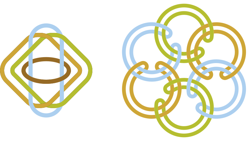
<p>While the three rings above—known as the <em>Borromean rings</em>—are especially simple and symmetric, similar links can be created for <em>any</em> number of rings. Here are links of four and six rings, for example, that fall apart if a single ring is removed:</p>

<p><br /></p>

<div style="text-align: center;">
    <img src="/assets/blogPics/brunnian_links.svg" width="500" alt="Brunnian links with four and six rings" />
</div>

<p><br /></p>

<p>I find this kind of magical. There seems to be a kind of ‘top-down’ causation: the behaviour of individual rings is restricted by the group as a whole, not by any individual. 
<br />
<br /></p>

<h2 id="making-sense-of-higher-order-structure">Making sense of higher-order structure</h2>
<p>The rings above are a simple example of a more general phenomenon known as ‘higher-order structure’ or ‘emergence’. These two terms are often used in an imprecise way. Imprecise use of ‘emergence’ does not bother me so much, because it seems to refer to something that is not very precise anyway (similar to ‘complexity’). But I believe that ‘higher-order structure’ can be made much more precise—it certainly sounds pretty mathematical. In fact, I recently wrote a paper about an idea that makes this precise, and that seems to explain many uses of the word ‘higher-order’. In particular, it answers the questions: <em>higher than what?</em> and <em>which order?</em> The paper is called <strong>A Mereological Approach to Higher-Order Structure in Complex Systems: from Macro to Micro with Möbius</strong> and is publicly available <a href="https://arxiv.org/pdf/2404.14423">here</a>. In this blog post<sup id="fnref:0" role="doc-noteref"><a href="#fn:0" class="footnote" rel="footnote">1</a></sup>, I hope to give a more accessible and less technical overview of the main ideas in the paper.</p>

<p><br />
<br /></p>

<h2 id="mereology">Mereology</h2>
<p>Mereology<sup id="fnref:1" role="doc-noteref"><a href="#fn:1" class="footnote" rel="footnote">2</a></sup> is the study of ‘parts’—specifically the relationship between parts and wholes. My central thesis is that incorporating mereology into scientific and mathematical thinking is a good idea. While a lot has been written about mereology—mostly by philosophers and logicians—it is not widely used as a practical set of ideas in the sciences. I suspect the aforementioned philosophers and logicians would find my approach simplistic, naive, or superficial, but I have found it to be very practical.</p>

<p><br /></p>

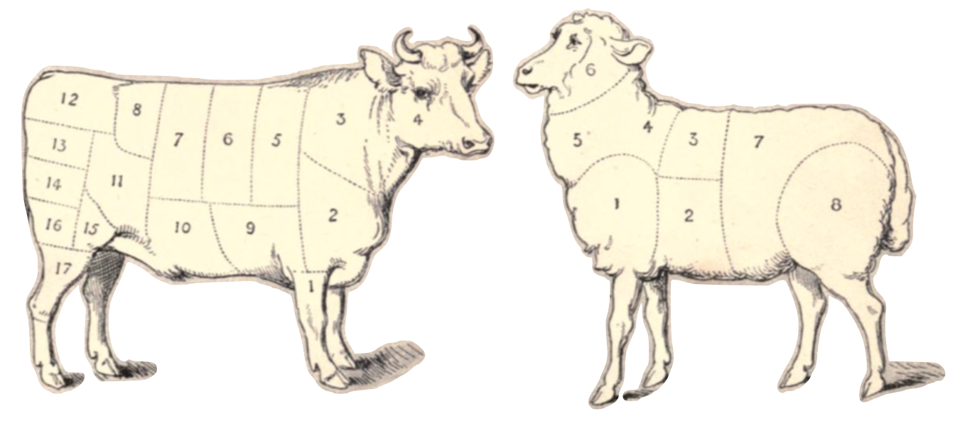
<p>If we want to describe parts and wholes, let’s start with the whole. It is the biggest possible part of itself. The whole can then be divided into smaller parts. One example of this is from the 1886 “Handbook of Practical Cookery” by Matilda Dods:</p>

<div style="text-align: center;">
    <img src="/assets/blogPics/ox_sheep.png" width="700" alt="Historic cutting diagrams of an ox and sheep" />
</div>

<p><br /></p>

<p>The parts can be further divided into smaller parts, and so on. It is natural to assume some rules that parts should obey:</p>

<p><br /></p>

<ul>
  <li>If $a$ is a part of $b$, and $b$ is a part of $c$, then $a$ is also a part of $c$.</li>
  <li>Every part is a part of itself (namely, the ‘trivial’ biggest possible part).</li>
  <li>If $a$ is a part of $b$, then $b$ is not a part of $a$ (unless $a=b$).</li>
</ul>

<p><br /></p>

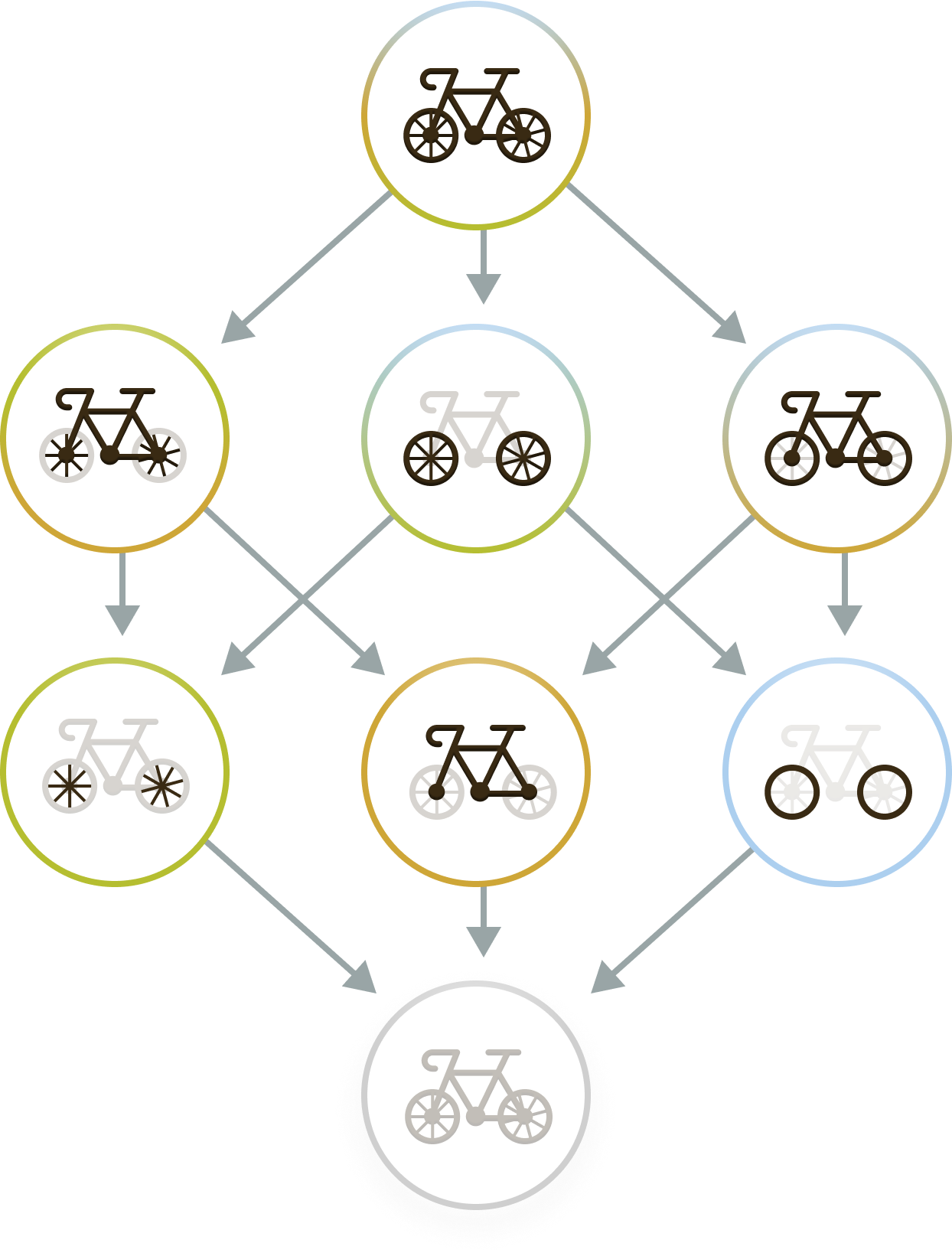
<p>These rules are well-known to mathematicians, who call them <em>transitivity</em>, <em>reflexivity</em>, and <em>antisymmetry</em>. Together, they define what is called a <em>partial order</em>. It gives a way to order a collection of things—in this case, wholes, parts, and parts of parts (and parts of parts of parts, etc.). When a part $a$ is smaller than (or equal to) part $b$, we write $a \leq b$. We say <em>partial</em> order, because not all parts can be put in order! A possible mereology on a bicycle is, for example, the following, where an arrow is drawn from a part $a$ to $b$ if $b$ is a part of $a$:</p>

<p><br /></p>

<div style="text-align: center;">
    <img src="/assets/blogPics/hasse_bicycle.png" width="400" alt="Mereological diagram of bicycle parts" />
</div>

<p><br /></p>

<p>Clearly, all the components drawn in black are ‘parts’ of the full bicycle, and the ordering reflects that the tires and the spokes are both parts of the wheels. However, the tires are not part of the frame, and <em>vice-versa</em>, so there is no arrow between the two—they are ‘incomparable’.</p>

<p><br /></p>

<p>Now let’s put on a more scientific hat. If we want to describe the mereology of a system, it makes sense to say that there is a <em>unique</em> part that is the biggest, namely the whole system. This is the <em>top</em> of the partial order of parts (for example, the fully assembled bicycle above). In addition, let’s assume that the system is only made up of a finite number of parts (a billion parts is fine, but infinitely many is not). If we call the system $S$, then I propose we call any (finite) partial order that has $S$ at the top a <em>mereology<sup id="fnref:2" role="doc-noteref"><a href="#fn:2" class="footnote" rel="footnote">3</a></sup> on $S$</em>. If we write the set of parts of $S$ as $\mathcal{D}(S)$ and the ordering as $\leq$, then the mereology can be summarised as the pair $(\mathcal{D}(S), \leq)$.</p>

<p><br />
<br /></p>

<h2 id="decomposing-complex-systems">Decomposing Complex Systems</h2>
<p>Fundamental to any description of Nature is the choice of parts. I imagine this like the cast of a theatre play: who are the characters that come together to tell the story. If you want to describe how an object behaves, you should decide whether you want to describe it in terms of the atoms, molecules, layers, structural elements, or something else. Once you make this choice, you can start writing down equations that describe how these parts interact. Say you want to predict some property of a system, let’s call it $Q$ for quantity. This could be the temperature of a material, or the height of a person—anything that can be described by a number is allowed here. If $Q$ is some macroscopic quantity that you could measure, then it makes sense to say: $Q(S)$ is the sum of microscopic contributions from all the parts that make up the system $S$. Since I’m imagining $Q$ to be an observable macroscopic quantity, built from microscopic contributions of the parts, I write them as a big $Q$ and little $q$ respectively. Each part can contribute something else, so I write $q(s)$ for the contribution of part $s$. Saying that the quantity $Q$ is the sum of the contributions of the parts can then be written mathematically as:</p>

\[Q(S) = \sum_{s \in S} q(s)\]

<p>Where I write $\sum\limits_{s \in S}$ to mean <em>“sum all the parts $s$ that are in $S$”</em>. Now the problem is that this can only really lead to very boring descriptions of the quantity $Q$. If the whole is just the sum of the parts, then your $Q$ is a pretty boring quantity. For example, say we want to describe the height of a person in terms of the genes they have. We could write this as $H(G)$: their height as a function of their genes. If then $H(G) = \sum\limits_{g \in G}h(g)$, then the height of a person is just determined independently by each gene. Biology is much more exciting than that: genes can individually contribute to your height, but they can also interact in complex ways and change each other’s effects. It therefore makes sense to extend our notion of <em>parts</em> to also include combinations of individual genes. For example, we could have contributions of three genes $g_1$, $g_2$, and $g_3$, but also of the pairs $(g_1, g_2)$, $(g_1, g_3)$, and $(g_2, g_3)$—and perhaps even the triplet $(g_1, g_2, g_3)$. Contributions from pairs are very common and usually called <em>interactions</em>. Less commonly considered is an interaction among three elements. Because interactions of more than two elements are less common, they are usually collectively referred to as <em>higher-order interactions</em><sup id="fnref:3" role="doc-noteref"><a href="#fn:3" class="footnote" rel="footnote">4</a></sup>.</p>

<p><br /></p>

<p>Ok let’s therefore assume that in principle, all parts <em>and all possible combinations</em> might contribute to the overall observation of $Q$ (though not all <em>have</em> to contribute—some contributions could be zero in practice). This means that the quantity $Q$ is not just the sum of the contributions of the parts, but also of the contributions of the pairs, triplets, quadruplets, and so on. This can be written as:</p>

\[Q(S) = \sum_{s \in S} q(s) + \sum_{\substack{s_1 \in S\\s_2 \in S}} q(s_1, s_2) + \sum_{\substack{s_1 \in S\\s_2 \in S\\s_3 \in S}} q(s_1, s_2, s_3) + \ldots\]

<p>To write this down more efficiently, we define the set of all possible combinations of parts of $S$ as $\mathcal{P}(S)$. Mathematicians call $\mathcal{P}(S)$ the <em>power set</em> of $S$. The quantity $Q$ can then be written as:</p>

\[Q(S) = \sum_{p \in \mathcal{P}(S)} q(p)\]

<p>We are now at the point where we can connect this back to mereology. Note that $\mathcal{P}(S)$ has an “order” to it. Let’s say $S = (g_1, g_2, g_3)$, then $\mathcal{P}(S) = (\emptyset, (g_1), (g_2), (g_3), (g_1, g_2), (g_1, g_3), (g_2, g_3), (g_1, g_2, g_3))$. The thing written as $\emptyset$ represents the ‘empty’ set $(~)$, which technically is also a part of $S$—namely the ‘empty part’. Note that some elements of $\mathcal{P}(S)$ can be made from others. For example, $(g_1, g_2)$ can be made from $(g_1)$ by adding $(g_2)$. In this sense, $(g_1)$ is a ‘part’ of $(g_1, g_2)$, and $(g_1, g_2)$ is thus “bigger” than $(g_1)$. This is usually written as $(g_1)\subseteq (g_1, g_2)$. It should not be too hard to convince yourself that $\mathcal{P}(S)$, ordered in this way by $\subseteq$, is a mereology on $S$!</p>

<p><br /></p>

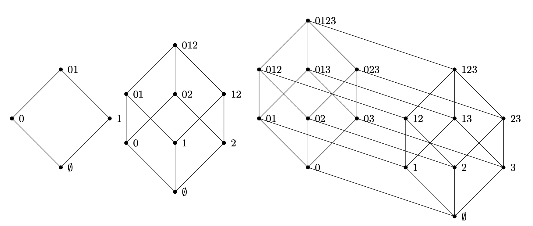
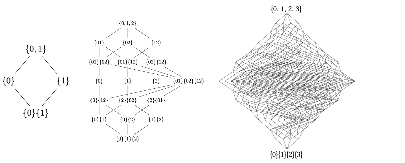
<p>Here’s a picture of the power set mereology on systems with 2, 3, or 4 variables (which I’ve labelled simply as $0$, $1$, $2$, and $3$):</p>

<div style="text-align: center;">
    <img src="/assets/blogPics/hasse_BAs.png" width="700" alt="Power set mereologies for systems with two, three, and four variables" />
</div>

<p><br /></p>

<p>Each has the full system at the top (as any mereology should), the empty set at the bottom, and in between all the singletons, pairs, triplets, and so on. All three also clearly have ‘levels’ or ‘orders’ corresponding to horizontal slices.</p>

<p>This means that we can now ‘decompose’ the quantity $Q(S)$ over a mereology on $S$ as follows</p>

\[Q(S) = \sum_{p \subseteq S} q(p)\]

<p>This now reads: $Q(S)$ is built from contributions from all the parts of $S$, including all possible combinations of them. Perhaps you are not yet convinced that we have gained anything by doing this. We have simply rewritten the decomposition of $Q$ in a more complicated form. However, mereologies have some special properties which allows us to do something pretty cool.</p>

<p><br /></p>

<h2 id="möbius-inversion">Möbius inversion</h2>
<p>Let’s leave the mereology unspecified for now, and just say there is some mereology $(\mathcal{D}(S), \leq)$ on $S$. The decomposition of $Q(S)$ can be written as:</p>

\[Q(S) = \sum_{p \leq S} q(p)\]

<p>By definition, every element of $\mathcal{D}(S)$ is a part of $S$. This means that if the full system $S$ has the property $Q(S)$, then any part $p$ might have the property $Q(p)$. Note that $Q(p)$ is not the same as $q(p)$—the former is a property of the part $p$, while the latter is the contribution of $p$ to the property of the whole system. Now it might make sense to say that the decomposition is valid for all parts:</p>

\[Q(p) = \sum_{r \leq p} q(r)\]

<p>This means that we have a decomposition of $Q$ on every part. If there is a total of $N$ parts in the mereology, then this leads to $N$ equations (one decomposition of $Q$ per part), with $N$ unknowns (the contribution $q$ of each part). This is a system of equations that could in theory be solved, but for large mereologies this can be impractical. Since a mereology is a very special thing with a lot of structure, solving the equations is actually much simpler! The solution is given by the <em>Möbius inversion formula</em>:</p>

\[Q(S) = \sum_{p \leq S} q(p) \quad \iff \quad q(S) = \sum_{p \leq S} \mu(p, S)Q(p)\]

<p>This says that whenever you have a sum over a mereology, you can actually invert this sum (‘solve the system of equations’). This gives you an expression for all the microscopic contributions $q(p)$, that are usually not directly observable, in terms of the observable properties of the parts $Q(r)$. $Q$ is a sum of $q$’s, but the $q$’s are themselves a sum of $Q$’s, weighed by a weird number called $\mu(p, S)$. This number is called the <em>Möbius function</em> of the mereology.</p>

<p><br /></p>

<p>The precise definition of $\mu$ is not so important<sup id="fnref:mf" role="doc-noteref"><a href="#fn:mf" class="footnote" rel="footnote">5</a></sup>. The only important thing is that it allows you to invert sums on a mereology, and that it is fully specified by the ‘shape’ of the mereology. Only the relationships between the parts matter—not what the parts actually <em>are</em>. For example, the power set mereology $(\mathcal{P}(S), \subseteq)$ that we saw before always has the same shape, no matter what kind of system $S$ is. This means that the Möbius function is always the same for the power set mereology. It is given by</p>

\[\mu(p, S) = (-1)^{|S| - |p|}\]

<p>In other words: if you decompose $Q(S)$ over the power set mereology, then the microscopic $q(p)$ given by an alternating sum over $Q(p)$’s:</p>

\[q(S) = \sum_{p \subseteq S} (-1)^{|S| - |p|}Q(p)\]

<p>Where $\mid S\mid - \mid p\mid$ refers to the difference in the number of elements in $S$ and $p$. Let’s look at two examples of this in practice.</p>

<p><br /></p>

<p><strong>Example 1</strong>: Consider a system of two genes $g_1$, and $g_2$. Let us decompose a person’s height $H$ over the power set mereology of these genes:</p>

\[H(g_1, g_2) = \sum_{p \subseteq (g_1, g_2)} h(p)
= {\color{grey}{h(\emptyset})} + {\color{YellowGreen}{h(g_1)}} + {\color{skyblue}{h(g_2)}} + {\color{Tan}{h(g_1, g_2)}}\]

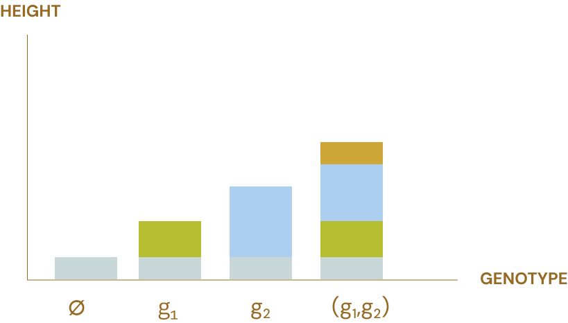
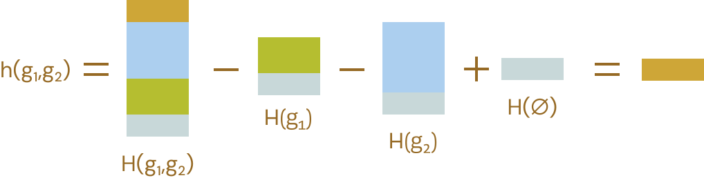
<p>This says: the height of the person with both genes is given by some contribution $h(\emptyset)$ that forms the ‘baseline’ height, plus the contributions of each gene individually, plus the interaction of the pair of genes. Matching the colour scheme above, we can draw this as:</p>

<div style="text-align: center;">
    <img src="/assets/blogPics/height_graph.svg" width="500" alt="Height contributions drawn on a two-gene power set diagram" />
</div>

<p>To infer the contribution of an individual gene, we apply the Möbius inversion formula:</p>

\[h(g_1) =  (-1)^{|g_1| - |g_1|}H(g_1) + (-1)^{|\emptyset| - |g_1|}H(\emptyset)\\
= H(g_1)- H(\emptyset)\]

<p>That is, the effect $h(g_1)$ of an individual gene is the difference between a person with that gene and a person without it. This makes sense! In fact, it makes so much sense that it is not very interesting. More interesting is the interaction term. A similar Möbius inversion yields:</p>

\[h(g_1, g_2) = H(g_1, g_2) - H(g_1) - H(g_2) + H(\emptyset)\]

<p>which can be drawn as:</p>

<p><br /></p>

<div style="text-align: center;">
    <img src="/assets/blogPics/height_inversion.svg" width="500" alt="Epistatic height contribution shown as an alternating sum" />
</div>

<p><br /></p>

<p>This is actually a well-known quantity in genetics, where it is known as an <em>epistatic effect</em> between the genes.</p>

<p><br /></p>

<p><strong>Example 2</strong> In physics and information theory, one often quantifies the amount of information in a system by the <em>entropy</em>. The precise definition is not important for now, but let’s denote the entropy carried by two variables $(X, Y)$ by $H(X, Y)$. One could imagine that the total entropy is composed of contributions from the individual variables, and a contribution that is only carried by the pair. This amounts to a power set mereology:</p>

\[H(X, Y) =  I(X) + I(Y) + I(X, Y)\]

<p>We have omitted the empty set this time, since an empty set of variables carries no information. A Möbius inversion shows that</p>

\[I(X, Y) = H(X, Y) - H(X) - H(Y)\]

<p>This is a quantity known as the <em>mutual information</em> between $X$ and $Y$, and represents one of the most fundamental concepts in information theory. While there are other ways to derive it, this shows that it is the <em>unique</em> way to decompose the entropy over subsets of variables.</p>

<p><br />
<br /></p>

<h2 id="beyond-power-sets">Beyond power sets</h2>
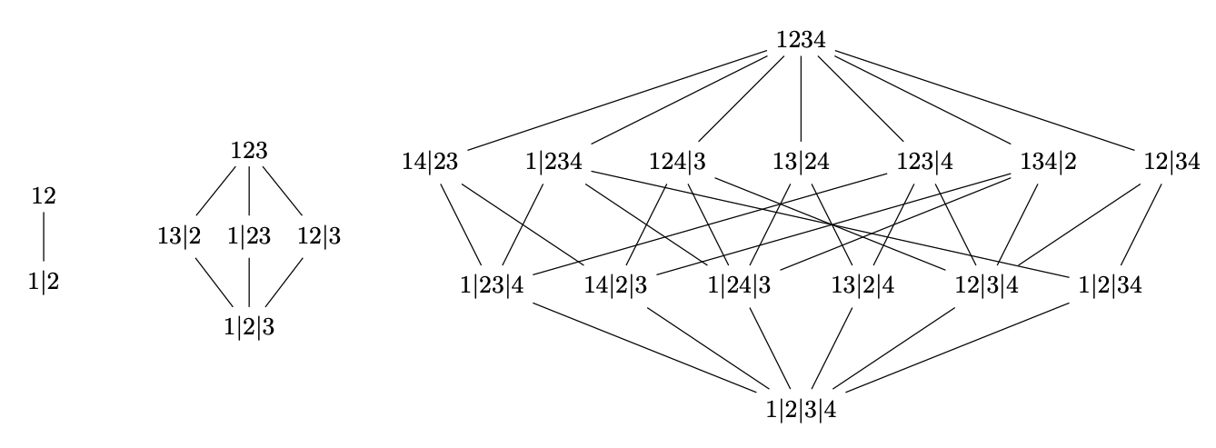
<p>Both examples above use the power set mereology, which is especially simple<sup id="fnref:4" role="doc-noteref"><a href="#fn:4" class="footnote" rel="footnote">6</a></sup>. In the paper, I find that Möbius inversions on different mereologies reproduce different quantities that are all well-known in certain fields of science. One alternative but common mereology is the ‘partition’ mereology, where a set is not divided into subsets, but into ‘partitions’—different ways to cut up a system. Here’s what that looks like for two, three, and four variables:</p>
<div style="text-align: center;">
    <img src="/assets/blogPics/hasse_partition.png" width="700" alt="Partition mereologies for systems with two, three, and four variables" />
</div>

<p><br /></p>

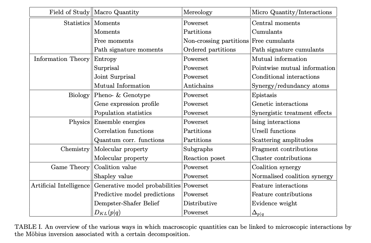
<p>Table 1 from the paper gives an overview of how different mereologies are associated to different quantities:</p>

<p><br /></p>

<div style="text-align: center;">
    <img src="/assets/blogPics/mereologies_table.png" width="900" alt="Table of mereologies and their associated scientific quantities" />
</div>

<p><br /></p>

<p>To summarise: Most of the quantities above were the result of people thinking very hard about what the right definition of the microscopic ‘interaction’ terms are. However, instead of thinking hard about equations, you can instead invest this mental energy into thinking about appropriate mereologies. Once you have fixed the mereology, there is a <em>unique</em> microscopic description that is compatible with it. Not only that, the mereology shows you exactly what is meant by ‘higher-order’, namely, some terms are higher with respect to the partial ordering. This resonates strongly with Plato’s call to ‘carve Nature at its joints’—a good description of Nature depends on a good choice of parts. If you choose a natural mereology, then the higher-order interactions that derive from it inherit the justification.</p>

<p><br /></p>

<h2 id="real-world-applications">Real-world applications</h2>
<p>In the paper I use this approach<sup id="fnref:5" role="doc-noteref"><a href="#fn:5" class="footnote" rel="footnote">7</a></sup> to derive new notions of ‘higher-order’ interactions that can be used in machine learning (I derive a novel decomposition of the so-called <em>KL-divergence</em>). Another exciting application is ‘coarse-graining’. Physicists <em>love</em> studying what happens when you ‘coarse-grain’ a system—how does the physics change if you squint or look from far away? In essence, a coarse-graining is simply a change in mereology—a coarser description is one with fewer or larger parts. Describing coarse-grainings at the level of mereologies gives an entirely new way to think about this process. In one of the final sections of the paper I show that coarse-grainings correspond to special kinds of transformations of mereologies called <em>Galois connections</em>, and use this to derive well-known coarse-grained quantities (the ‘renormalised’ Ising couplings).</p>

<p><br /></p>

<p>To apply the framework, you have to know the Möbius function $\mu$ of the mereology you are interested in. For one famous mereology—the so-called redundancy mereology—the Möbius function was not known. It is a particularly complex mereology and includes <em>many</em><sup id="fnref:dedekind" role="doc-noteref"><a href="#fn:dedekind" class="footnote" rel="footnote">8</a></sup> parts:</p>
<div style="text-align: center;">
    <img src="/assets/blogPics/hasse_antichains.png" width="700" alt="Redundancy mereology Hasse diagram for four variables" />
</div>

<p><br /></p>

<p>However, in a recent collaboration with Pedro Mediano at Imperial College London, and Fernando Rosas at Sussex, we were able to calculate the Möbius function for this mereology, and therefore calculate new kinds of higher-order interactions (see the paper <a href="https://arxiv.org/pdf/2410.06224">here</a>). I’m now exploring what else can be done with this approach, and recently found a new way to decompose causal effects, as outlined <a href="https://arxiv.org/pdf/2501.11447">here</a>.</p>

<p><br /></p>

<p><strong>In short: there is lots to do. Stay tuned for more.</strong></p>

<p><br /> 
<br /></p>

<div class="footnotes" role="doc-endnotes">
  <ol>
    <li id="fn:0" role="doc-endnote">
      <p><span style="color:grey">Thanks to Twitter/X user <a href="https://x.com/prathyvsh">@prathyvsh</a> for urging me to write this, and creating the figures of Brunnian links and visual algebra. They make <a href="https://x.com/prathyvsh/status/1790097597107241210">really great visualisations of algebraic structures</a></span> <a href="#fnref:0" class="reversefootnote" role="doc-backlink">&#8617;</a></p>
    </li>
    <li id="fn:1" role="doc-endnote">
      <p><span style="color:grey">Mereology is the <em>λόγος</em> (logos: explanation/consideration) of a <em>μέρος</em> (meros: part). The <em>meros</em> root more famously appears in words like <em>polymer</em> (literally: manyparts).</span> <a href="#fnref:1" class="reversefootnote" role="doc-backlink">&#8617;</a></p>
    </li>
    <li id="fn:2" role="doc-endnote">
      <p><span style="color:grey">Mathematicians might notice how this is somewhat similar to the definition of a <em>topology</em>. The two are indeed related, but not the same. A topology on a finite set is necessarily a mereology, but not all mereologies are topologies, and topologies do not have to be finite. </span> <a href="#fnref:2" class="reversefootnote" role="doc-backlink">&#8617;</a></p>
    </li>
    <li id="fn:3" role="doc-endnote">
      <p><span style="color:grey">It’s interesting to ask: <em>Why</em> are beyond-pairwise interactions not common? I think it’s at least part caused by a lack of imagination. We can picture things interacting as a graph, where points represent parts, and lines represent interactions between parts. But lines always connect two points, not three or more, so we cannot really picture what higher-order interactions look like. This is a limitation of our imagination, not of Nature. However, pairwise descriptions have been very successful, and some people have argued that this is the way Nature works. Observing higher-order interactions from data is also harder than pairwise interactions, so perhaps it is simply a reflection of the fact that data sets have historically been small. This would also explain why higher-order interactions are becoming more <em>en vogue</em> now that data sets are getting bigger. </span> <a href="#fnref:3" class="reversefootnote" role="doc-backlink">&#8617;</a></p>
    </li>
    <li id="fn:mf" role="doc-endnote">
      <p><span style="color:grey">The Möbius function is usually recursively defined over a partial order, but there is a very nice expression due to Phillip Hall: Given an interval $[x, y]$ on the partial order $P$, let $c_i$ be the number of chains in $P$ from $x$ to $y$ of length $i$. Then the Möbius function on $P$ is given by $\mu(x, y) = -c_1 + c_2 - c_3 + \ldots$. </span> <a href="#fnref:mf" class="reversefootnote" role="doc-backlink">&#8617;</a></p>
    </li>
    <li id="fn:4" role="doc-endnote">
      <p><span style="color:grey">The Möbius inversion formula over the power set mereology is more famously known as the <em>inclusion-exclusion principle</em>.</span> <a href="#fnref:4" class="reversefootnote" role="doc-backlink">&#8617;</a></p>
    </li>
    <li id="fn:5" role="doc-endnote">
      <p><span style="color:grey">I’m still looking for a good name for this approach/framework. Möreology? If you have any suggestions—please let me know!</span> <a href="#fnref:5" class="reversefootnote" role="doc-backlink">&#8617;</a></p>
    </li>
    <li id="fn:dedekind" role="doc-endnote">
      <p><span style="color:grey">In fact, the number of parts in this mereology for 9 variables was calculated for the first time in 2023, and for more than 9 variables is still unknown.</span> <a href="#fnref:dedekind" class="reversefootnote" role="doc-backlink">&#8617;</a></p>
    </li>
  </ol>
</div>]]></content><author><name>Abel Jansma</name></author><category term="physics" /><category term="biology" /><category term="cybernetics" /><category term="causality" /><category term="game-theory" /><category term="maths" /><category term="philosophy" /><category term="machine-learning" /><category term="information-theory" /><summary type="html"><![CDATA[]]></summary></entry><entry><title type="html">The Encyclopedia of Mobius Inversions in the Sciences</title><link href="https://abeljansma.nl/2025/01/28/encycloMobius.html" rel="alternate" type="text/html" title="The Encyclopedia of Mobius Inversions in the Sciences" /><published>2025-01-28T08:00:00+00:00</published><updated>2025-01-28T08:00:00+00:00</updated><id>https://abeljansma.nl/2025/01/28/encycloMobius</id><content type="html" xml:base="https://abeljansma.nl/2025/01/28/encycloMobius.html"><![CDATA[<p><br />
<br /></p>

<p>In a <a href="https://journals.aps.org/prresearch/abstract/10.1103/PhysRevResearch.7.023016">recent paper</a>, I proposed to study complex systems through a mereological lens by applying the Möbius inversion theorem. I also covered this in <a href="/2025/01/28/mereoPhysics.html">a recent blogpost</a>. Here, I will collect some of the most important applications of Möbius transformations in the sciences. I will update this table as I find more applications. If you have suggestions, please send me an email, or leave a comment below!</p>

<p><br />
<br /></p>

<table>
  <thead>
    <tr>
      <th>Field of Study</th>
      <th>Macro quantity</th>
      <th>Mereology</th>
      <th>Micro quantity</th>
    </tr>
  </thead>
  <tbody>
    <tr>
      <td><strong>Statistics</strong></td>
      <td>Moments</td>
      <td>Powerset</td>
      <td>Central moments</td>
    </tr>
    <tr>
      <td> </td>
      <td>Moments</td>
      <td>Partitions</td>
      <td>Cumulants</td>
    </tr>
    <tr>
      <td> </td>
      <td>Free moments</td>
      <td>Non-crossing partitions</td>
      <td>Free cumulants</td>
    </tr>
    <tr>
      <td> </td>
      <td>Path signature moments</td>
      <td>Ordered partitions</td>
      <td>Path signature cumulants</td>
    </tr>
    <tr>
      <td> </td>
      <td>Causal effects</td>
      <td>Antichains</td>
      <td>Causal synergy/redundancy</td>
    </tr>
    <tr>
      <td><strong>Information Theory</strong></td>
      <td>Entropy</td>
      <td>Powerset</td>
      <td>Mutual information</td>
    </tr>
    <tr>
      <td> </td>
      <td>Entropy</td>
      <td>Singletons</td>
      <td>Total correlation</td>
    </tr>
    <tr>
      <td> </td>
      <td>Surprisal</td>
      <td>Powerset</td>
      <td>Pointwise mutual information</td>
    </tr>
    <tr>
      <td> </td>
      <td>Joint Surprisal</td>
      <td>Powerset</td>
      <td>Conditional interactions</td>
    </tr>
    <tr>
      <td> </td>
      <td>Mutual Information</td>
      <td>Antichains</td>
      <td>Synergy/redundancy atom</td>
    </tr>
    <tr>
      <td><strong>Biology</strong></td>
      <td>Pheno- &amp; Genotype</td>
      <td>Powerset</td>
      <td>Epistasis</td>
    </tr>
    <tr>
      <td> </td>
      <td>Gene expression profile</td>
      <td>Powerset</td>
      <td>Genetic interactions</td>
    </tr>
    <tr>
      <td> </td>
      <td>Population statistics</td>
      <td>Powerset</td>
      <td>Synergistic treatment effect</td>
    </tr>
    <tr>
      <td><strong>Physics</strong></td>
      <td>Energy</td>
      <td>Powerset</td>
      <td>Ising interactions</td>
    </tr>
    <tr>
      <td> </td>
      <td>Correlation functions</td>
      <td>Partitions</td>
      <td>Ursell functions</td>
    </tr>
    <tr>
      <td> </td>
      <td>Quantum corr. functions</td>
      <td>Partitions</td>
      <td>Scattering amplitudes</td>
    </tr>
    <tr>
      <td><strong>Chemistry</strong></td>
      <td>Molecular property</td>
      <td>Subgraphs</td>
      <td>Fragment contributions</td>
    </tr>
    <tr>
      <td> </td>
      <td>Molecular property</td>
      <td>Reaction poset</td>
      <td>Cluster contributions</td>
    </tr>
    <tr>
      <td><strong>Game Theory</strong></td>
      <td>Coalition value</td>
      <td>Powerset</td>
      <td>Harsanyi dividends</td>
    </tr>
    <tr>
      <td> </td>
      <td>Shapley value</td>
      <td>Supersets</td>
      <td>Normalised coalition synergy</td>
    </tr>
    <tr>
      <td><strong>Artificial Intelligence</strong></td>
      <td>Generative model probabilities</td>
      <td>Powerset</td>
      <td>Feature interaction</td>
    </tr>
    <tr>
      <td> </td>
      <td>Predictive model predictions</td>
      <td>Powerset</td>
      <td>Feature contribution</td>
    </tr>
    <tr>
      <td> </td>
      <td>Dempster-Shafer Belief</td>
      <td>Lattices</td>
      <td>Evidence weight</td>
    </tr>
    <tr>
      <td> </td>
      <td>KL-divergence</td>
      <td>Powerset</td>
      <td>$\Delta_{p|q}$ measure</td>
    </tr>
  </tbody>
</table>]]></content><author><name>Abel Jansma</name></author><category term="physics" /><category term="biology" /><category term="cybernetics" /><category term="causality" /><category term="game-theory" /><category term="maths" /><category term="philosophy" /><category term="machine-learning" /><category term="information-theory" /><summary type="html"><![CDATA[]]></summary></entry><entry><title type="html">A Möbius inversion theorem for modules and vector spaces</title><link href="https://abeljansma.nl/2025/01/28/moduleMobius.html" rel="alternate" type="text/html" title="A Möbius inversion theorem for modules and vector spaces" /><published>2025-01-28T08:00:00+00:00</published><updated>2025-01-28T08:00:00+00:00</updated><id>https://abeljansma.nl/2025/01/28/moduleMobius</id><content type="html" xml:base="https://abeljansma.nl/2025/01/28/moduleMobius.html"><![CDATA[<p><br /></p>

<p>In a <a href="/2025/01/28/mereoPhysics.html">previous post</a>, I proposed to study complex systems through a mereological lens by applying the Möbius inversion theorem. This has become my favourite theorem by now, because I think it allows you to do integration and differentiation on observables in complex systems where this was not possible before.</p>

<p><br /></p>

<p>It was originally proved by Möbius for integer numbers ordered by division, but generalised to commutative rings and arbitrary posets by Gian-Carlo Rota. I wanted to apply this to group- and vector-valued functions so that I could calculate semantic synergy in text embeddings, but to do so the theorem needed to be generalised. Let’s first review the classical version of the theorem, and then generalise it to modules and vector spaces.</p>

<p><br /></p>

<p><strong>Definition:</strong> A commutative ring $R$ (with unity) is a set equipped with two operations, addition ($+$) and multiplication ($\cdot$), such that the following properties hold:</p>

<p>    1. $(R, +)$ is an Abelian group with identity element $0_R$.</p>

<p>    2. $(R, \cdot)$ is a monoid with identity element $1_R$.</p>

<p>    3. Multiplication distributes over addition: $a \cdot (b + c) = a \cdot b + a \cdot c$ and $(a + b) \cdot c = a \cdot c + b \cdot c$</p>

<p>    4. Multiplication is commutative: $a \cdot b = b \cdot a$</p>

<p><br /></p>

<h2 id="the-classical-möbius-inversion-theorem">The Classical Möbius Inversion Theorem</h2>
<p>The theorem is really a statement about the <em>incidence algebra</em> of the poset $P$, which is the set of all functions $f: P \times P \to R$ from intervals on $P$ to $R$, equipped with the convolution product defined by:</p>

\[(f \ast g)(x, y) = \sum_{x\leq z \leq y} f(x, z) \cdot g(z, y)\]

<p>Note that the following three functions are part of the incidence algebra:</p>

\[\begin{align}
\zeta(x, y) &amp;= \begin{cases}
1_R &amp; \text{if } x \leq y \\
0_R &amp; \text{otherwise} \\
\end{cases} \\[1em]
\mu(x, y) &amp;= \begin{cases}
1_R &amp; \text{if } x = y \\
 -\sum_{x \leq z &lt; y} \mu(x, z) &amp; \text{if } x &lt; y \\
0_R &amp; \text{otherwise}
\end{cases} \\[1em]
\delta(x, y) &amp;= \begin{cases}
1_R &amp; \text{if } x = y \\
0_R &amp; \text{otherwise}\\
\end{cases}
\end{align}\]

<p><strong>Theorem (Möbius inversion theorem):</strong> Let $R$ be a commutative ring, and $f, g: P \to R$ be $R$-valued functions defined on a locally finite poset $P$. Then the following two statements are equivalent:</p>

<p>    1. $f(x) = \sum_{y \leq x} g(y)$</p>

<p>    2. $g(x) = \sum_{y \leq x} \mu(y, x) \cdot f(y)$</p>

<p>where $\mu$ is the Möbius function on $P$.</p>

<p><br /></p>

<p>The Möbius inversion theorem is thus really the statement that $\mu$ is the $\ast$-inverse of $\zeta$, as $\zeta \ast \mu = \delta$ and $\mu \ast \zeta = \delta$. This is a very powerful result: since $f$ is like an integral over the poset, $\mu$ is like a differential operator on $P$.</p>

<p><br /></p>

<h2 id="generalising-the-möbius-inversion-theorem">Generalising the Möbius Inversion Theorem</h2>

<p>It turns out that we can generalise this theorem to group-valued functions. This is strictly more general than the commutative ring case, and includes vector-valued functions. To do so, we need to define $R$-modules:</p>

<p><br /></p>

<p><strong>Definition:</strong> Let $R$ be a commutative ring. An <em>R-module</em> is an Abelian group $M$ with a group operation $\oplus : M \times M \to M$ and a scalar multiplication $\star: R \times M \to M$ such that the following properties hold for all $r, s \in R$ and $x, y \in M$:</p>

<p>    1. $r \star (x \oplus y) = r \star x \oplus r \star y$</p>

<p>    2. $(r + s) \star x = r \star x \oplus s \star x$</p>

<p>    3. $r \star (s \star x) = (r \cdot s) \star x$</p>

<p>    4. $1 \star x = x$</p>

<p><br /></p>

<p>We can then state a more general version of the theorem:</p>

<p><br /></p>

<p><strong>Theorem (Möbius inversion theorem on R-modules):</strong> Let $(P, \leq)$ be a locally finite poset, $(R, +, \cdot)$ a commutative ring, and $(M, \oplus,\star)$ an R-module. Consider $Q, q: P \to M$. Then the following two statements are equivalent:</p>

<p>    1. $Q(x) = \bigoplus_{y \leq x} q(y)$</p>

<p>    2. $q(x) = \bigoplus_{y \leq x} \mu(y, x) \star Q(y)$</p>

<p><br /></p>

<p><strong><em>Proof:</em></strong> The proof is similar to the classical case, but we need to carefully consider the properties of the different operations involved.</p>

<p>Filling in the first statement into the right-hand side of the second statement:</p>

\[\bigoplus_{y \leq x} \mu(y, x) \star Q(y) = \bigoplus_{y \leq x} \left( \mu(y, x) \star \bigoplus_{z \leq y} q(z) \right)\]

<p>By the first property of modules,  $\star$ multiplication distributes over $\oplus$ addition:</p>

\[= \bigoplus_{y \leq x} \left(\bigoplus_{z \leq y} \mu(y, x) \star q(z) \right)\]

<p>As the module is based on an Abelian group, $\bigoplus$ is associative and commutative, so we can change the order of summation as follows:</p>

\[= \bigoplus_{z \leq x} \left( \bigoplus_{z\leq y \leq x} \mu(y, x) \star q(z) \right)\]

<p>By the second property of modules, we can replace the $\bigoplus$ (addition in the group) with $\sum$ (addition in the ring) as follows:</p>

\[= \bigoplus_{z \leq x} \left( \sum_{z\leq y \leq x} \mu(y, x) \right) \star q(z)\]

<p>Observe that the term in parentheses is equal to $(\zeta \ast \mu)(z, x)=\delta(z, x)$, a convolution in the incidence algebra. Therefore:</p>

\[= \bigoplus_{z \leq x} \delta(z, x) \star q(z) = 1_R \star q(x) = q(x)\]

<p>This proves that the second statement follows from the first.</p>

<p>To prove the reverse direction, we fill in the second statement into the first:</p>

\[\bigoplus_{y \leq x} q(y) = \bigoplus_{y \leq x} \left( \bigoplus_{z \leq y} \mu(z, y) \star Q(z) \right)\]

<p>From here, the same arguments can be applied to show that this equals $Q(x)$. This completes the proof. $\square$</p>

<p><br /></p>

<h2 id="conclusion">Conclusion</h2>

<p>The theorem is thus no longer a statement about convolutions in the incidence algebra, but about a kind of ‘incidence action’ on the module. This generalisation opens up new possibilities for applying Möbius inversion to group- or vector-valued function. One context in which this might be useful is text embeddings. The Möbius inverse of the vector-valued embedding function would quantify the ‘emergent semantics’ of a piece of text.</p>]]></content><author><name>Abel Jansma</name></author><category term="maths" /><summary type="html"><![CDATA[]]></summary></entry><entry><title type="html">Möbius Functions on Powerset Antichains</title><link href="https://abeljansma.nl/2024/02/09/antichains.html" rel="alternate" type="text/html" title="Möbius Functions on Powerset Antichains" /><published>2024-02-09T14:00:00+00:00</published><updated>2024-02-09T14:00:00+00:00</updated><id>https://abeljansma.nl/2024/02/09/antichains</id><content type="html" xml:base="https://abeljansma.nl/2024/02/09/antichains.html"><![CDATA[<p>UPDATE: I have now found an explicit formula for the Möbius function on the redundancy lattice. This will appear in a preprint soon.</p>

<p><br /></p>

<p>I calculated the full Möbius function on the lattice of powerset antichains of 2, 3, and 4 variables. As far as I can tell, these results have not been shared before, although I’m sure the 2- and 3-variable case has been calculated but not shared many times before. The results and the code are available <a href="https://github.com/AJnsm/latticeOfAntichains">here</a>.</p>

<p><br /></p>

<p>This should make higher-order information decompositions much more straightforward and computationally efficient when one is interested in more than 3 variables. Some background information on what this is all means is given below.</p>

<p><br /></p>

<p>Given a set $S$, the powerset $\mathcal{P}(S)$ is the set of all subsets of $S$. From this set, one can create a partially ordered set $P=(\mathcal{P}(S), \leq)$, where we impose the following ordering. For $s, t \in \mathcal{P}(S)$, we say that $s \leq t$ if and only if $s \subseteq t$. This is a partial ordering because not all pairs of elements are comparable. For example, if $S=\{1,2,3\}$, then $\{1\}$ and $\{2\}$ are not comparable, but it’s clear that $\{1\} \leq \{1,2\}$.</p>

<p><br /></p>

<p>Now one can imagine functions $f: P^n \to \mathbb{C}$ on this poset. Of particular interest is the so-called Möbius function $\mu: P^2 \to \mathbb{N}$, which is defined recursively:</p>

\[\mu(s,t) = \begin{cases}
1 &amp; \text{if } s = t \\
-\sum_{s &lt; u \leq t} \mu(u, t) &amp; \text{if } s &lt; t\\
0 &amp; \text{otherwise }\\
\end{cases}\]

<p>This function is important because it allows the Möbius inversion theorem (due to Rota, 1964) to be stated:</p>

\[f(t) = \sum_{s \leq t} g(s) \Leftrightarrow g(t) = \sum_{s \leq t} \mu(s,t) f(s)\]

<p>This theorem forms the basis for our understanding of interactions in complex systems (more details in an upcoming manuscript).</p>

<p><br /></p>

<p>The Möbius function is most studied on the following posets:</p>
<ul>
  <li>The poset $(\mathbb{N}, \leq)$ of natural number with their natural ordering (in which case the Möbius inversion theorem reduces to the discrete fundamental theorem of calculus)</li>
  <li>The poset $(\mathbb{N}, \leq_d)$ of natural numbers ordered by divisibility (in which case $\mu$ is the inverse of the Riemann zeta function)</li>
  <li>On the poset $(\mathcal{P}, \subseteq)$ of subsets ordered by inclusion (in which case $\mu(s, t)=(-1)^{\mid t-s \mid }$)</li>
  <li>On the poset $(\Pi(S), \leq_r)$ of partitions of a set $S$ ordered by refinement (in which case $\mu(\pi, S)=(-1)^{(\pi-1)}(\mid \pi\mid -1)!$).</li>
</ul>

<p><br /></p>

<p>Here, however, I will focus a much less understood poset, inspired by a branch of information theory called the Partial Information Decomposition (PID). The PID aims to decompose information into unique, redundant, and synergistic components. The key insight is that given a set of variables, one can define redundant information quantities that depend on particular combinations of the variables. The central constraint is that the redundant information should only be nontrivial for two sets of variables that are incomparable on the poset of subsets $P$ defined above. This is because a redundancy among $A$ and $B$ is only meaningful if $A$ is not a subset of $B$ (or <em>vice versa</em>).</p>

<p><br /></p>

<p>Now, an important observation is that the collection of these incomparable subsets have an interesting structure. A collection of incomparable items is called an <em>antichain</em> (because it is in some sense the opposite of a chain on $P$), and antichains can again be given a partial order! Let’s call the collection of antichains $A$, so that for every $a, b \in A$, we can set  $a \leq b$ if for every $b_i \in b$, there is an $a_i \in a$ such that $a_i \subseteq b_i$. That is, $b$ in some sense ‘covers’ $a$, and $b$ contains less redundancy than $a$.</p>

<p><br /></p>

<p>The partial information decomposition then writes the total information a set of sources $X_1 \ldots X_n$ carries about a target $Y$ as a sum of <em>information atoms</em> $\Pi$ on this lattice of antichains:</p>

\[I(\{X_1, \ldots, X_n\}; Y) = \sum_{a \in A} \Pi(a; Y)\]

<p>To identify what the information atoms are in terms of already known information quantities, we can interpret $I(\{X_1, \ldots, X_n\}; Y)$ as a function $I: A \to \mathbb{R}$, and then apply the Möbius inversion theorem to find the information atoms $\Pi(a; Y)$.</p>

<p><br /></p>

<p>The problem is that we don’t have a closed form solution for the Möbius function on $A$. If we did, we could calculate arbitrary information atoms and pinpoint exactly which parts of a system show synergistic information processing. In addition, a brute-force calculation is very hard, as the number of antichains grows superexponentially with the number of variables. In fact, the number of antichains on a set of $n$ variables is given by the $n$’th Dedekind number (minus two), which is <a href="https://oeis.org/A000372">a series</a> that grows so fast that only the first nine terms are known: 2, 3, 6, 20, 168, 7581, 7828354, 2414682040998, 56130437228687557907788, 286386577668298411128469151667598498812366. That last term was, in fact, <a href="https://www.uni-paderborn.de/en/news-item/123917">first calculated in 2023</a>.</p>

<p><br /></p>

<p>Still, one would only need to calculate the Möbius functions on the lattice of antichains once, after which any time you want to decompose some information quantity you can just look up the value. Because this sequence grows so quickly, the literature has so far only really calculated decompositions of the information that two variables carry about a third. I wrote some code that calculates the Möbius function on the lattice of antichains (available <a href="https://github.com/AJnsm/latticeOfAntichains">on Github</a>), and have stored the results for up to 4 variables giving information about a fifth. This is not a huge improvement, but it’s a start, and I invite anyone to see how far they can optimise my code and perhaps calculate higher Möbius functions (it’s currently a <a href="https://github.com/AJnsm/latticeOfAntichains/blob/main/calcMF_antichains.py">pretty basic Python implementation</a>). I’m pretty sure the 5-variable case is doable with my current approach, but beyond that it looks like more clever approaches have to be found.</p>

<p><br /></p>

<p>I found that the Möbius function on the lattice of antichains, up to $N=4$, only takes the values $-1$, $0$, and $1$. This is similar to Möbius functions on other posets, like Boolean algebras or positive integers ordered by divisibility, but this does not mean that finding a closed form expression for the Möbius function will be easy. For example, the Möbius function on the positive number orders by divisibility also only takes values -1, 0, and 1, but a closed form expression would solve the Riemann hypothesis and win you a million dollars. Still, I suspect that the Möbius function on the lattice of antichains is more tractable than one might think, since there seems to be a close relationship between the product of antichain lattices and Boolean algebras, for which the Möbius function is well understood.</p>

<p><br /></p>

<p>The main advantage of having these Möbius functions calculated is that new PID approaches now no longer need to solve the system of equations each time a new definition of redundancy is introduced, and can instead use the Möbius function to calculate all information atoms directly. Especially as the number of variables grows, solving the system of PID equations becomes increasingly hard, so having stored values of the Möbius function can offer a huge advantage.</p>]]></content><author><name>Abel Jansma</name></author><category term="information-theory" /><category term="maths" /><category term="cybernetics" /><summary type="html"><![CDATA[UPDATE: I have now found an explicit formula for the Möbius function on the redundancy lattice. This will appear in a preprint soon.]]></summary></entry><entry><title type="html">Introducing: Stator</title><link href="https://abeljansma.nl/2023/12/21/Stator.html" rel="alternate" type="text/html" title="Introducing: Stator" /><published>2023-12-21T14:00:00+00:00</published><updated>2023-12-21T14:00:00+00:00</updated><id>https://abeljansma.nl/2023/12/21/Stator</id><content type="html" xml:base="https://abeljansma.nl/2023/12/21/Stator.html"><![CDATA[<p>In my <a href="/../assets/JansmaAbel_PhDThesis_corrected.pdf">PhD thesis</a>, I developed a method and software package to infer interactions and cell states from gene expression data. Both the <a href="https://github.com/AJnsm/Stator">software</a> and the <a href="https://www.biorxiv.org/content/10.1101/2023.12.18.572232">research</a> are now published!</p>

<p>The software is called Stator, and comprises the <a href="https://github.com/AJnsm/Stator">Stator Nextflow pipeline</a>, as well as a bespoke <a href="https://shiny.igc.ed.ac.uk/MFIs/">Shiny app</a> developed by Yuelin Yao.</p>

<p><br /></p>

<p><a href="https://www.biorxiv.org/content/10.1101/2023.12.18.572232">We used it</a> to find previously hidden differentiation states in the embryonic mouse brain and sub-phases of the cell cycle, and discovered liver tumour cell states that are prognostic of patient survival. Please get in touch if you are interested in using Stator for your own research!</p>

<p><br /></p>

<p><img src="/assets/research_info/CC_states.png" alt="Image of a combinatorial gene regulation" width="600" /></p>]]></content><author><name>Abel Jansma</name></author><category term="biology" /><category term="causality" /><category term="maths" /><category term="cybernetics" /><summary type="html"><![CDATA[In my PhD thesis, I developed a method and software package to infer interactions and cell states from gene expression data. Both the software and the research are now published!]]></summary></entry><entry><title type="html">A simple origami swallow</title><link href="https://abeljansma.nl/2023/09/02/origami-swallow.html" rel="alternate" type="text/html" title="A simple origami swallow" /><published>2023-09-02T08:00:00+00:00</published><updated>2023-09-02T08:00:00+00:00</updated><id>https://abeljansma.nl/2023/09/02/origami-swallow</id><content type="html" xml:base="https://abeljansma.nl/2023/09/02/origami-swallow.html"><![CDATA[<p>I was completely mesmerised by the swallows in Portugal, and while playing around with some origami paper, I came up with this simple design for an origami swallow. It is based on the famous ‘crane base’ (steps 1-7), and implements many folds used in the standard Orizuru crane (inside-reverse folds for the wings, narrowing the bottom two flaps, etc).</p>

<h2 id="step-1">Step 1</h2>

<p>Two diagonal valley folds, and two horizontal mountain folds.</p>

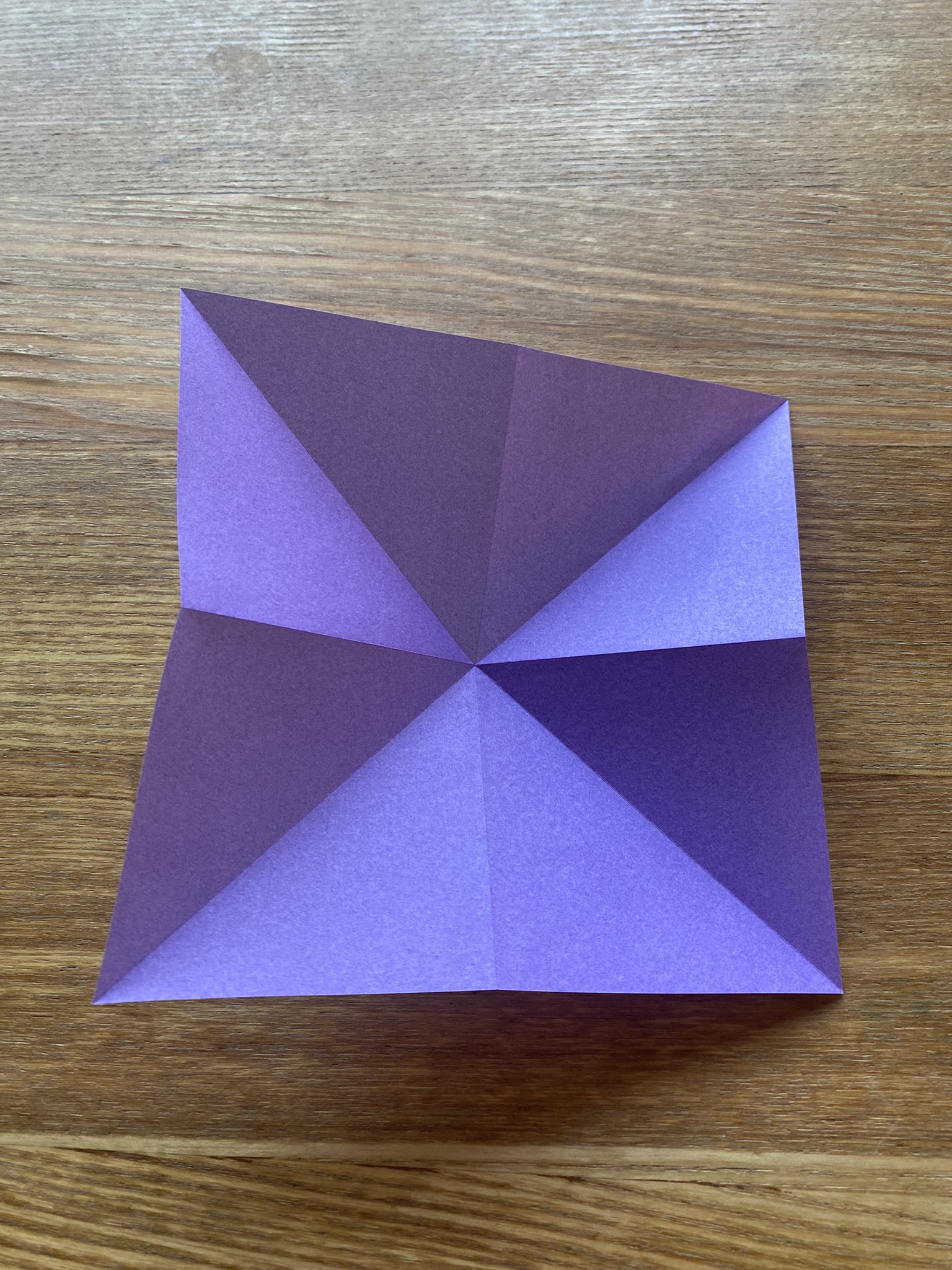
<p><img src="/assets/origami_swallow/step1.jpeg" alt="Step1" width="250" /></p>

<p><br /></p>

<h2 id="step-2">Step 2</h2>

<p>Push the diagonals together along the valley folds.</p>

<p><img src="/assets/origami_swallow/step2.jpeg" alt="Step2" width="250" /></p>

<p><br /></p>

<h2 id="step-3">Step 3</h2>

<p>Flatten, keep the open sides at the bottom.</p>

<p><img src="/assets/origami_swallow/step3.jpeg" alt="Step3" width="250" /></p>

<p><br /></p>

<h2 id="step-4">Step 4</h2>

<p>Fold the open edges inwards (on both sides).</p>

<p><img src="/assets/origami_swallow/step4.jpeg" alt="Step4" width="250" /></p>

<p><br /></p>

<h2 id="step-5">Step 5</h2>

<p>Fold the top triangle down.</p>

<p><img src="/assets/origami_swallow/step5.jpeg" alt="Step5" width="250" /></p>

<p><br /></p>

<h2 id="step-6">Step 6</h2>

<p>Undo the previous fold.</p>

<p><img src="/assets/origami_swallow/step6.jpeg" alt="Step6" width="250" /></p>

<p><br /></p>

<h2 id="step-7">Step 7</h2>

<p>Open the two flaps and fold the inside triangle up (on both sides).</p>

<p><img src="/assets/origami_swallow/step7.jpeg" alt="Step7" width="250" /></p>

<p><br /></p>

<h2 id="step-8">Step 8</h2>

<p>Open the four sides.</p>

<p><img src="/assets/origami_swallow/step8.jpeg" alt="Step8" width="250" /></p>

<p><br /></p>

<h2 id="step-9">Step 9</h2>

<p>Close and flatten along the edges previously not touching.</p>

<p><img src="/assets/origami_swallow/step9.jpeg" alt="Step9" width="250" /></p>

<p><br /></p>

<h2 id="step-10">Step 10.</h2>

<p>Fold along the bottom diagonals.</p>

<p><img src="/assets/origami_swallow/step10.jpeg" alt="Step10" width="250" /></p>

<p><br /></p>

<h2 id="step-11">Step 11.</h2>

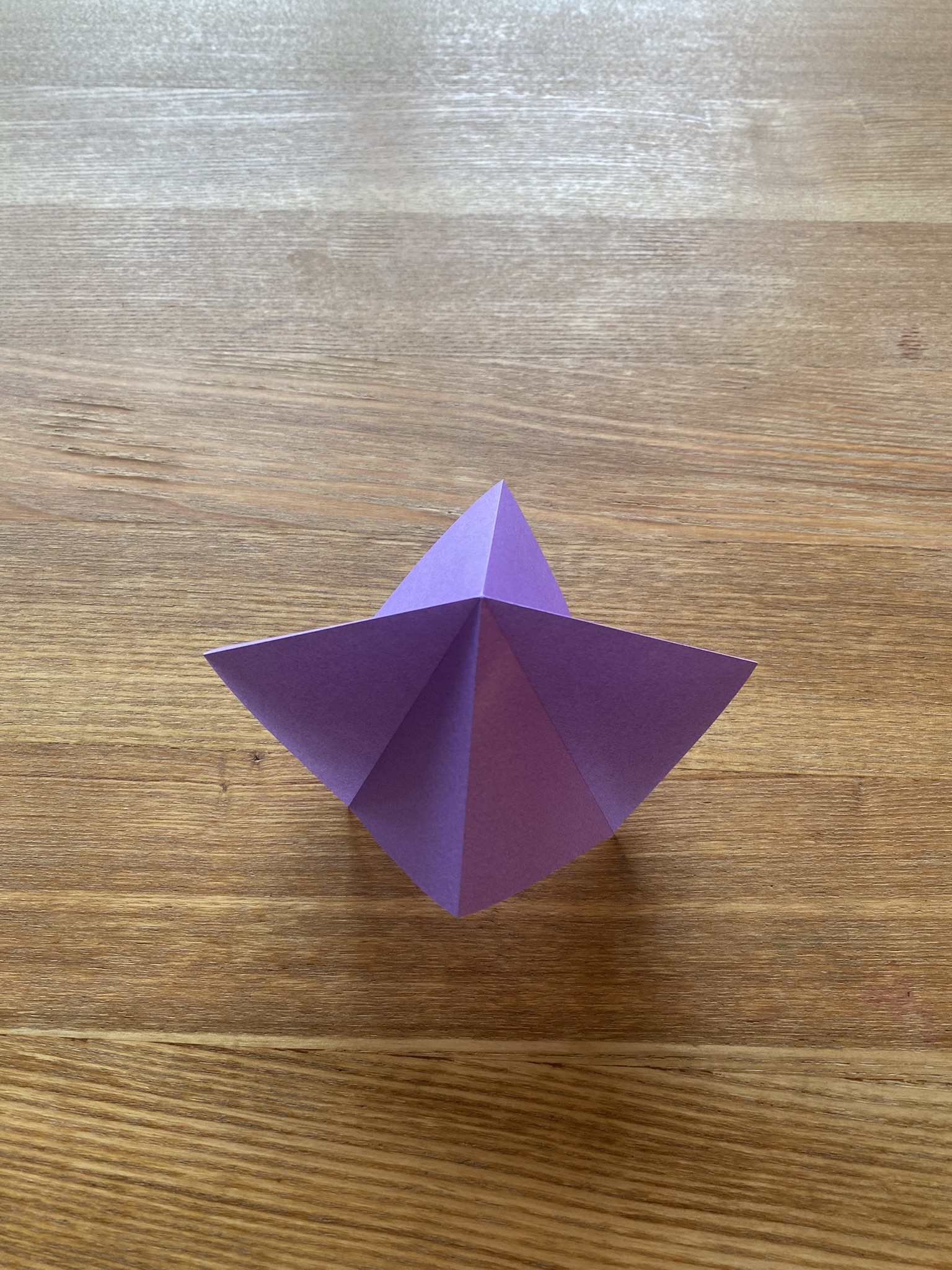
<p>Open the two wings with an inside reverse fold. This is a free fold that determines the angle of the wings.</p>

<p><img src="/assets/origami_swallow/step11.jpeg" alt="Step11" width="250" /></p>

<p><br /></p>

<h2 id="step-12">Step 12.</h2>

<p>Fold open the v-shaped tail. This is another free fold.</p>

<p><img src="/assets/origami_swallow/step12.jpeg" alt="Step12" width="250" /></p>

<p><br /></p>]]></content><author><name>Abel Jansma</name></author><category term="miscellaneous" /><summary type="html"><![CDATA[I was completely mesmerised by the swallows in Portugal, and while playing around with some origami paper, I came up with this simple design for an origami swallow. It is based on the famous ‘crane base’ (steps 1-7), and implements many folds used in the standard Orizuru crane (inside-reverse folds for the wings, narrowing the bottom two flaps, etc).]]></summary></entry><entry><title type="html">The do-calculus of sampling from restricted Boltzmann machines</title><link href="https://abeljansma.nl/2023/01/09/RBMs-and-DoCalculus.html" rel="alternate" type="text/html" title="The do-calculus of sampling from restricted Boltzmann machines" /><published>2023-01-09T08:00:00+00:00</published><updated>2023-01-09T08:00:00+00:00</updated><id>https://abeljansma.nl/2023/01/09/RBMs-and-DoCalculus</id><content type="html" xml:base="https://abeljansma.nl/2023/01/09/RBMs-and-DoCalculus.html"><![CDATA[<p>Generative models, in particular energy-based models, are often used to sample from conditional distributions–a process known as <em>inpainting</em>. One of the most fundamental kinds of generative energy-based models is called a restricted Boltzmann machine (RBM), which is essentially a bipartite, glassy Ising model. Inpainting with RBMs is usually done by sampling from the visible layer while fixing the value of some visible nodes, which is an <em>intervention</em>, not a passive observation. I could not find a proof that the resulting interventional sampling distribution approaches the conditional distribution, so here follows an argument that it in fact does (in the case of Gibbs sampling), based on the do-calculus.</p>

<p><br /></p>

<p>Given a Bayesian network of variables $V$ represented by a DAG $G = (V, E)$, the fundamental problem in causal inference is to estimate quantities like $p_G\left(V_A=v_a \mid do(V_B=v_b)\right)$ for an arbitrary partition of the vertices $V = V_A \cup V_B$. The do-calculus provides rules and methods for answering such questions. Unfortunately, the standard formulation of RBMs is not suitable for treatment by the do-calculus, as the network of dependencies does not form a DAG. However, by exploiting the sequential nature of Gibbs-sampling, I show the following:</p>

<p><br /></p>

<p><strong>Lemma</strong> (RBM inpainting is conditional sampling) 
Consider a restricted Boltzmann machine with visible nodes $v$ and hidden nodes $h$, where $|v|&gt;0$ and $|h|&gt;0$. Let $p(v)$ be the marginal probability distribution over the visible nodes, and $v = v_a \cup v_b$ an arbitrary partition of the visible nodes. Consider the nodes of the RBM as random variables that evolve under alternating Gibbs sampling of the visible and the hidden layers. Define the do-operator on a variable $X$ as fixing that variable $X=x$ before generating each sample, and the see-operator as passively observing $X=x$. Then:</p>

\[p(v_a | do(v_b)) = p(v_a | see(v_b)) = p(v_a | v_b)~~~~~~~~~~~~~~~~ (1)\]

<p>That is, inpainting is sampling from the conditional distribution.</p>

<p><em>(proof)</em>
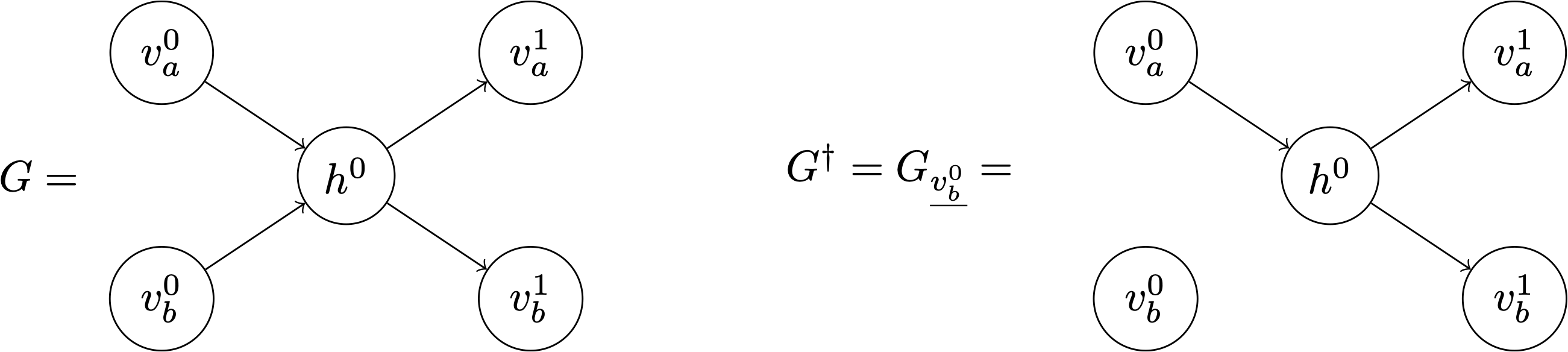
First note that the RBM has to be represented by a DAG. To do this, consider the nodes as random variables that evolve under Gibbs sampling. The bipartite structure of the network allows us to unroll the network in time:</p>

<p><br /></p>

<p><img src="/assets/blogPics/unrolled.png" alt="" /></p>

<p><br /></p>

<p>where $v^i$ and $h^i$ mark the $i$’th Gibbs sample of the visible and hidden layer, respectively. Given the partition $v = v_a \cup v_b$, the following should be verified:</p>

\[p(v^1_a \mid do(v^0_b)) = p(v^1_a \mid v^0_b) ~~~~~~~~~~~~~~~~ (2)\]

<p>The second rule of the do-calculus states:</p>

<p><br /></p>

<p><strong>Rule 2</strong>(Action/observation exchange)</p>

\[p(y \mid do(x), do(z), w) = p(y \mid do(x), z, w) \text{ if } (Y\!\perp\!\!\!\perp Z \mid X, W)_{G_{\overline{X}\underline{Z}}}\]

<p>where $G_{\overline{X}\underline{Z}}$ is the graph $G$ with all the arrows into $X$, and out of $Z$ removed. If $X=W=\emptyset$, then Rule 2 can be directly apply to Equation (1) by defining the following two graphs:</p>

<p><br /></p>

<p><img src="/assets/blogPics/interventionGraphs.png" alt="" /></p>

<p><br /></p>

<p>where $v$ could be partitioned because at any given time point the visible nodes are mutually independent conditional on the hidden layer. The value of $v_b^1$ will be discarded and set to $v_b^0$ again, but that is irrelevant in the present discussion. Now 
\((v_a^1 \!\perp\!\!\!\perp v_b^0)_{G^\dagger}\), which by <strong>Rule 2</strong> implies Equation (2), and completes the proof. $\square$</p>

<p><br /></p>

<p><br /></p>

<p><strong>Example</strong> As a very simple example, consider the case where $v_a=v_1$, $v_b=v_2$ and $h_1$ all comprise just a single node. The full distribution is:</p>

\[P_G(v_1, v_2, h_1) = \frac{1}{\mathcal{Z}_G} e^{h_1 w_{11} v_1 + h_1 w_{12} v_2 + b_1 v_1 + b_2 v_2 + c_1 h_i}\]

<p>Denoting by $(abc)$ the situation in which $v_1=a, ~v_2=b, ~h_1=c$, the conditional distribution after observing $v_2=1$ is:</p>

<p><br /></p>

\[\begin{align*}
    P(v_1=1|\text{see}(v_2=1)) &amp;= \frac{P_G(v_1=1, v_2=1)}{P_G(v_2=1)}\\
    &amp;= \frac{(110) + (111)}{(111) + (110) + (011) + (010)}\\
    &amp;= \frac{e^{b_1+b_2} + e^{w_{11} + w_{12} + b_1 + b_2 + c_1}}{e^{w_{11}+w{12}+b_1+b_2+c_1} + e^{b_1+b_2} + e^{w_{12} + b_2 + c_1} + e^{b_2}}\\
    &amp;= \frac{e^{b_1} + e^{w_{11} + w_{12} + b_1  + c_1}}{e^{w_{11}+w{12}+b_1+c_1} + e^{b_1} + e^{w_{12}  + c_1} + 1} 
\end{align*}\]

<p><br /></p>

<p>Now consider the intervention $do(v_2=1)$. It just adds a bias $w_{12}$ to the hidden layer. Denoting by $(ab)$ that $v_1=a, ~h_1=b$:</p>

<p><br /></p>

\[\begin{align*}
    P_G(v_1=1|\text{do}(v_2=1)) &amp;= P_{G^\dagger}(v_1=1)\\
        &amp;= \frac{1}{\mathcal{Z}_{G^\dagger}} \Big((11) + (10)\Big) 
\end{align*}\]

<p><br /></p>

<p>Writing out this partition function:</p>

<p><br /></p>

\[\mathcal{Z}_{G^\dagger} = (11) + (10) + (01) + (00)
    = e^{w_{11}+b_1+c_1+w_{12}} + e^{b_1} + e^{c_1+w_{12}} + 1\]

<p><br /></p>

<p>so that</p>

<p><br /></p>

\[P(v_1=1|\text{do}(v_2=1)) = \frac{e^{w_{11}+b_1+c_1+w_{12}} + e^{b_1}}{e^{w_{11}+b_1+c_1+w_{12}} + e^{b_1} + e^{c_1+w_{12}} + 1}\]

<p>which indeed coincides with expression for the see-operator.</p>]]></content><author><name>Abel Jansma</name></author><category term="machine-learning" /><category term="causality" /><category term="maths" /><category term="dualities-in-statistics" /><summary type="html"><![CDATA[Generative models, in particular energy-based models, are often used to sample from conditional distributions–a process known as inpainting. One of the most fundamental kinds of generative energy-based models is called a restricted Boltzmann machine (RBM), which is essentially a bipartite, glassy Ising model. Inpainting with RBMs is usually done by sampling from the visible layer while fixing the value of some visible nodes, which is an intervention, not a passive observation. I could not find a proof that the resulting interventional sampling distribution approaches the conditional distribution, so here follows an argument that it in fact does (in the case of Gibbs sampling), based on the do-calculus.]]></summary></entry><entry><title type="html">Using the Open Game engine to model MEV</title><link href="https://abeljansma.nl/2022/12/15/EPF8.html" rel="alternate" type="text/html" title="Using the Open Game engine to model MEV" /><published>2022-12-15T08:00:00+00:00</published><updated>2022-12-15T08:00:00+00:00</updated><id>https://abeljansma.nl/2022/12/15/EPF8</id><content type="html" xml:base="https://abeljansma.nl/2022/12/15/EPF8.html"><![CDATA[<p><span style="color:grey">(This is an update on my Ethereum Protocol Fellowship. More updates can be found <a href="/2022/10/18/EPF0.html">here</a> ).</span></p>

<p><br /></p>

<h2 id="extracting-value-from-uniswap-transactions">Extracting value from Uniswap transactions</h2>

<p>In this post, I will outline a way in which the equilibrium analysis from the Open Game engine can be used to come up with profitable strategies for a block proposer on the Ethereum blockchain, either by re-ordering the transactions in the block, or by inserting their own. I will consider two sources of MEV here, inspired by the <a href="https://arxiv.org/abs/2109.04347">Clockwork Finance paper</a>. First, I will consider transactions to a Uniswap-like exchange, that exchanges two tokens according to the <a href="https://github.com/runtimeverification/verified-smart-contracts/blob/uniswap/uniswap/x-y-k.pdf">constant product rule</a>. By ordering such transactions, the block proposer can profitably manipulate the price of the tokens. Second, such price manipulation can be made even more profitable by placing a bet on the exchange rate offered by the Uniswap contract. To be able to analyse both these scenarios, I will model a blockchain with just two player accounts, $p_0$ and $p_1$, and two contract accounts: Uniswap and Bet. Most of the complexity will be captured in Haskell functions, and the Open Game engine is only used to search for profitable strategies for the block proposer $p_0$.</p>

<p><br /></p>

<p>Let’s first define some useful data types. I assume there exist only two tokens: <code class="language-plaintext highlighter-rouge">A</code> and <code class="language-plaintext highlighter-rouge">B</code>, both of which can be held in fractional amounts. An <code class="language-plaintext highlighter-rouge">Account</code> has an integer <code class="language-plaintext highlighter-rouge">AccountID</code>, and can hold amounts of both tokens. A transaction <code class="language-plaintext highlighter-rouge">Tx</code> specifies a sender and receiver ID, and how much of which token is sent. A block is simply modelled as a list of transactions:</p>

<p><br /></p>

<div class="language-haskell highlighter-rouge"><div class="highlight"><pre class="highlight"><code><span class="kr">data</span> <span class="kt">Token</span> <span class="o">=</span> <span class="kt">A</span> <span class="o">|</span> <span class="kt">B</span>
  <span class="kr">deriving</span> <span class="p">(</span><span class="kt">Eq</span><span class="p">,</span><span class="kt">Ord</span><span class="p">,</span><span class="kt">Show</span><span class="p">)</span>
<span class="kr">type</span> <span class="kt">TokenAmount</span> <span class="o">=</span> <span class="kt">Double</span>
<span class="kr">type</span> <span class="kt">AccountID</span> <span class="o">=</span> <span class="kt">Int</span>

<span class="c1">-- ID, amount A, amount B</span>
<span class="kr">type</span> <span class="kt">Account</span> <span class="o">=</span> <span class="p">(</span><span class="kt">AccountID</span><span class="p">,</span> <span class="kt">TokenAmount</span><span class="p">,</span> <span class="kt">TokenAmount</span><span class="p">)</span>

<span class="kr">type</span> <span class="kt">AccountStates</span> <span class="o">=</span> <span class="p">[</span><span class="kt">Account</span><span class="p">]</span>

<span class="c1">-- Sender, Receiver, Token, Amount</span>
<span class="c1">-- Should this also have a data field?</span>
<span class="kr">type</span> <span class="kt">Tx</span> <span class="o">=</span> <span class="p">(</span><span class="kt">AccountID</span><span class="p">,</span> <span class="kt">AccountID</span><span class="p">,</span> <span class="kt">Token</span><span class="p">,</span> <span class="kt">TokenAmount</span><span class="p">)</span>

<span class="kr">type</span> <span class="kt">TxBlock</span> <span class="o">=</span> <span class="p">[</span><span class="kt">Tx</span><span class="p">]</span>
</code></pre></div></div>

<p><br /></p>

<p>Let’s further define useful functions to find the recipient of a transaction and to set and get an account’s balance:</p>

<p><br /></p>

<div class="language-haskell highlighter-rouge"><div class="highlight"><pre class="highlight"><code><span class="n">getReceiver</span> <span class="o">::</span> <span class="kt">Tx</span> <span class="o">-&gt;</span> <span class="kt">AccountID</span>
<span class="n">getReceiver</span> <span class="p">(</span><span class="kr">_</span><span class="p">,</span><span class="n">receiver</span><span class="p">,</span> <span class="kr">_</span><span class="p">,</span> <span class="kr">_</span><span class="p">)</span> <span class="o">=</span> <span class="n">receiver</span>

<span class="n">balance</span> <span class="o">::</span> <span class="kt">Account</span> <span class="o">-&gt;</span> <span class="kt">Token</span> <span class="o">-&gt;</span> <span class="kt">TokenAmount</span>
<span class="n">balance</span> <span class="p">(</span><span class="n">userID</span><span class="p">,</span> <span class="n">amountA</span><span class="p">,</span> <span class="n">amountB</span><span class="p">)</span> <span class="n">token</span>
    <span class="o">|</span> <span class="n">token</span><span class="o">==</span><span class="kt">A</span> <span class="o">=</span> <span class="n">amountA</span>
    <span class="o">|</span> <span class="n">otherwise</span> <span class="o">=</span>  <span class="n">amountB</span>

<span class="n">updateAccount</span> <span class="o">::</span> <span class="kt">Account</span> <span class="o">-&gt;</span> <span class="kt">Token</span> <span class="o">-&gt;</span> <span class="kt">TokenAmount</span> <span class="o">-&gt;</span> <span class="kt">Account</span>
<span class="n">updateAccount</span> <span class="p">(</span><span class="n">acID</span><span class="p">,</span> <span class="n">bA</span><span class="p">,</span> <span class="n">bB</span><span class="p">)</span> <span class="n">token</span> <span class="n">amount</span>
   <span class="o">|</span> <span class="n">token</span> <span class="o">==</span> <span class="kt">A</span> <span class="o">=</span> <span class="p">(</span><span class="n">acID</span><span class="p">,</span> <span class="n">bA</span> <span class="o">+</span> <span class="n">amount</span><span class="p">,</span> <span class="n">bB</span><span class="p">)</span>
   <span class="o">|</span> <span class="n">otherwise</span> <span class="o">=</span> <span class="p">(</span><span class="n">acID</span><span class="p">,</span> <span class="n">bA</span><span class="p">,</span> <span class="n">bB</span> <span class="o">+</span> <span class="n">amount</span><span class="p">)</span>
</code></pre></div></div>

<p><br /></p>

<p>A call to the Uniswap contract is a map from the current state and a transaction to a new state. To generate the new state from the old one, I use a lens on the list, imported from <code class="language-plaintext highlighter-rouge">Control.Lens</code>. When a user has insufficient funds, they are charged a small (gas) fee.</p>

<p><br /></p>

<div class="language-haskell highlighter-rouge"><div class="highlight"><pre class="highlight"><code><span class="n">uniSwapExchange</span> <span class="o">::</span> <span class="kt">AccountStates</span> <span class="o">-&gt;</span> <span class="kt">Tx</span> <span class="o">-&gt;</span> <span class="kt">AccountStates</span>
<span class="c1">-- Old state -&gt; transaction -&gt; new state</span>
<span class="c1">-- Use lenses to 'modify' account states</span>
<span class="c1">-- If the user does not have sufficient funds, fine the user (a gas fee?) propagate the old state</span>
<span class="n">uniSwapExchange</span> <span class="n">accountStates</span> <span class="p">(</span><span class="n">userID</span><span class="p">,</span> <span class="n">uniSwapID</span><span class="p">,</span> <span class="n">token</span><span class="p">,</span> <span class="n">tokenAmount</span><span class="p">)</span>
   <span class="o">|</span> <span class="n">userbalanceInsufficient</span> <span class="o">=</span> <span class="n">accountStates</span> <span class="o">&amp;</span> <span class="p">(</span><span class="n">ix</span> <span class="n">userID</span><span class="p">)</span> <span class="o">.~</span> <span class="n">userFined</span>
   <span class="o">|</span> <span class="n">otherwise</span> <span class="o">=</span> <span class="n">accountStates</span> <span class="o">&amp;</span> <span class="p">(</span><span class="n">ix</span> <span class="n">userID</span><span class="p">)</span> <span class="o">.~</span> <span class="n">userUpdate</span> <span class="o">&amp;</span> <span class="p">(</span><span class="n">ix</span> <span class="n">uniSwapID</span><span class="p">)</span> <span class="o">.~</span> <span class="n">uniswapUpdate</span>
  <span class="kr">where</span>
   <span class="n">user_bal</span> <span class="o">=</span> <span class="n">balance</span> <span class="p">(</span><span class="n">accountStates</span><span class="o">!!</span><span class="n">userID</span><span class="p">)</span>
   <span class="n">userbalanceInsufficient</span> <span class="o">=</span> <span class="n">user_bal</span> <span class="n">token</span> <span class="o">&lt;</span> <span class="n">tokenAmount</span>
   <span class="n">userFined</span> <span class="o">=</span> 
      <span class="kr">if</span> <span class="n">token</span> <span class="o">==</span><span class="kt">A</span>
      <span class="kr">then</span> <span class="p">(</span><span class="n">userID</span><span class="p">,</span> <span class="n">minimum</span> <span class="p">[</span><span class="mi">0</span><span class="p">,</span> <span class="n">user_bal</span> <span class="kt">A</span> <span class="o">-</span> <span class="mf">0.1</span><span class="p">]</span> <span class="p">,</span> <span class="n">user_bal</span> <span class="kt">B</span><span class="p">)</span>
      <span class="kr">else</span> <span class="p">(</span><span class="n">userID</span><span class="p">,</span> <span class="n">user_bal</span> <span class="kt">A</span> <span class="p">,</span>  <span class="n">minimum</span> <span class="p">[</span><span class="mi">0</span><span class="p">,</span> <span class="n">user_bal</span> <span class="kt">B</span> <span class="o">-</span> <span class="mf">0.1</span><span class="p">])</span>
   <span class="n">uniSwap_bal</span> <span class="o">=</span> <span class="n">balance</span> <span class="p">(</span><span class="n">accountStates</span><span class="o">!!</span><span class="n">uniSwapID</span><span class="p">)</span>
   <span class="n">dA</span> <span class="o">=</span> <span class="n">uniSwap_bal</span> <span class="kt">A</span> <span class="o">*</span> <span class="n">tokenAmount</span> <span class="o">/</span> <span class="p">(</span><span class="n">uniSwap_bal</span> <span class="kt">B</span> <span class="o">+</span> <span class="n">tokenAmount</span><span class="p">)</span> 
   <span class="n">dB</span> <span class="o">=</span> <span class="n">uniSwap_bal</span> <span class="kt">B</span> <span class="o">*</span> <span class="n">tokenAmount</span> <span class="o">/</span> <span class="p">(</span><span class="n">uniSwap_bal</span> <span class="kt">A</span> <span class="o">+</span> <span class="n">tokenAmount</span><span class="p">)</span> 
   <span class="n">userUpdate</span> <span class="o">=</span> 
      <span class="kr">if</span> <span class="n">token</span> <span class="o">==</span> <span class="kt">A</span>
      <span class="kr">then</span> <span class="p">(</span><span class="n">userID</span><span class="p">,</span> <span class="n">user_bal</span> <span class="kt">A</span> <span class="o">-</span> <span class="n">tokenAmount</span><span class="p">,</span> <span class="n">user_bal</span> <span class="kt">B</span> <span class="o">+</span> <span class="n">dB</span><span class="p">)</span>
      <span class="kr">else</span> <span class="p">(</span><span class="n">userID</span><span class="p">,</span> <span class="n">user_bal</span> <span class="kt">A</span> <span class="o">+</span> <span class="n">dA</span><span class="p">,</span> <span class="n">user_bal</span> <span class="kt">B</span> <span class="o">-</span> <span class="n">tokenAmount</span><span class="p">)</span>
   <span class="n">uniswapUpdate</span> <span class="o">=</span> 
      <span class="kr">if</span> <span class="n">token</span> <span class="o">==</span> <span class="kt">A</span>
      <span class="kr">then</span> <span class="p">(</span><span class="n">uniSwapID</span><span class="p">,</span> <span class="n">uniSwap_bal</span> <span class="kt">A</span> <span class="o">+</span> <span class="n">tokenAmount</span><span class="p">,</span> <span class="n">uniSwap_bal</span> <span class="kt">B</span> <span class="o">-</span> <span class="n">dB</span><span class="p">)</span>
      <span class="kr">else</span> <span class="p">(</span><span class="n">uniSwapID</span><span class="p">,</span> <span class="n">uniSwap_bal</span> <span class="kt">A</span> <span class="o">-</span> <span class="n">dA</span><span class="p">,</span> <span class="n">uniSwap_bal</span> <span class="kt">B</span> <span class="o">+</span> <span class="n">tokenAmount</span><span class="p">)</span>
</code></pre></div></div>

<p><br /></p>

<p>Similarly, a call to the Bet contract transforms an old state into a new one, but it also needs an <code class="language-plaintext highlighter-rouge">AccountID</code> that specifies which contract should be used as a price oracle. It further needs the price that would trigger a win for the better. Crucially, both of these are a property of the contract, and not set by the transaction that actually places a bet of a certain amount. I’ve implemented it so that when the user wins a bet in token T, they receive the full T-balance of the betting contract.</p>

<p><br /></p>

<div class="language-haskell highlighter-rouge"><div class="highlight"><pre class="highlight"><code><span class="n">betOnExchange</span> <span class="o">::</span> <span class="kt">AccountStates</span> <span class="o">-&gt;</span> <span class="kt">AccountID</span> <span class="o">-&gt;</span> <span class="kt">Double</span> <span class="o">-&gt;</span> <span class="kt">Tx</span> <span class="o">-&gt;</span> <span class="kt">AccountStates</span>
<span class="c1">-- Old state, price oracle, bet threshold, bet amount, new state</span>
<span class="c1">-- Use lenses to 'modify' account states</span>
<span class="n">betOnExchange</span> <span class="n">accountStates</span> <span class="n">oracleID</span> <span class="n">ratio</span> <span class="p">(</span><span class="n">userID</span><span class="p">,</span> <span class="n">betID</span><span class="p">,</span> <span class="n">betToken</span><span class="p">,</span> <span class="n">betAmount</span><span class="p">)</span>
   <span class="o">|</span> <span class="p">(</span><span class="n">userbalanceInsufficient</span> <span class="o">||</span> <span class="n">betAmount</span><span class="o">&lt;</span><span class="mi">0</span><span class="p">)</span> <span class="o">=</span> <span class="n">accountStates</span> <span class="o">&amp;</span> <span class="p">(</span><span class="n">ix</span> <span class="n">userID</span><span class="p">)</span> <span class="o">.~</span> <span class="n">userFined</span>
   <span class="o">|</span> <span class="p">((</span><span class="n">uniSwap_bal</span> <span class="kt">A</span><span class="p">)</span><span class="o">/</span><span class="p">(</span><span class="n">uniSwap_bal</span> <span class="kt">B</span><span class="p">)</span> <span class="o">&gt;=</span> <span class="n">ratio</span><span class="p">)</span> <span class="o">=</span> <span class="n">accountStates</span> <span class="o">&amp;</span> <span class="p">(</span><span class="n">ix</span> <span class="n">userID</span><span class="p">)</span> <span class="o">.~</span> <span class="n">userUpdate_userWin</span> <span class="o">&amp;</span> <span class="p">(</span><span class="n">ix</span> <span class="n">betID</span><span class="p">)</span> <span class="o">.~</span> <span class="n">betUpdate_userWin</span>
   <span class="o">|</span> <span class="p">((</span><span class="n">uniSwap_bal</span> <span class="kt">A</span><span class="p">)</span><span class="o">/</span><span class="p">(</span><span class="n">uniSwap_bal</span> <span class="kt">B</span><span class="p">)</span> <span class="o">&lt;</span>  <span class="n">ratio</span><span class="p">)</span> <span class="o">=</span> <span class="n">accountStates</span> <span class="o">&amp;</span> <span class="p">(</span><span class="n">ix</span> <span class="n">userID</span><span class="p">)</span> <span class="o">.~</span> <span class="n">userUpdate_userLose</span> <span class="o">&amp;</span> <span class="p">(</span><span class="n">ix</span> <span class="n">betID</span><span class="p">)</span> <span class="o">.~</span> <span class="n">betUpdate_userLose</span>
  <span class="kr">where</span>
   <span class="n">uniSwap_bal</span> <span class="o">=</span> <span class="n">balance</span> <span class="p">(</span><span class="n">accountStates</span><span class="o">!!</span><span class="n">oracleID</span><span class="p">)</span>
   <span class="n">bet_bal</span> <span class="o">=</span> <span class="n">balance</span> <span class="p">(</span><span class="n">accountStates</span><span class="o">!!</span><span class="n">betID</span><span class="p">)</span>
   <span class="n">user_bal</span> <span class="o">=</span> <span class="n">balance</span> <span class="p">(</span><span class="n">accountStates</span><span class="o">!!</span><span class="n">userID</span><span class="p">)</span>
   <span class="n">userbalanceInsufficient</span> <span class="o">=</span> <span class="n">user_bal</span> <span class="n">betToken</span> <span class="o">&lt;</span> <span class="n">betAmount</span>
   <span class="n">userFined</span> <span class="o">=</span> 
      <span class="kr">if</span> <span class="n">betToken</span> <span class="o">==</span><span class="kt">A</span>
      <span class="kr">then</span> <span class="p">(</span><span class="n">userID</span><span class="p">,</span> <span class="n">minimum</span> <span class="p">[</span><span class="mi">0</span><span class="p">,</span> <span class="n">user_bal</span> <span class="kt">A</span> <span class="o">-</span> <span class="mf">0.1</span><span class="p">]</span> <span class="p">,</span> <span class="n">user_bal</span> <span class="kt">B</span><span class="p">)</span>
      <span class="kr">else</span> <span class="p">(</span><span class="n">userID</span><span class="p">,</span> <span class="n">user_bal</span> <span class="kt">A</span> <span class="p">,</span>  <span class="n">minimum</span> <span class="p">[</span><span class="mi">0</span><span class="p">,</span> <span class="n">user_bal</span> <span class="kt">B</span> <span class="o">-</span> <span class="mf">0.1</span><span class="p">])</span>
   <span class="c1">-- The prize is either the amount bet, or the remaining balance if that is less</span>
   <span class="n">prize</span> <span class="o">=</span> <span class="n">minimum</span> <span class="p">[</span><span class="n">betAmount</span><span class="p">,</span> <span class="n">balance</span> <span class="p">(</span><span class="n">accountStates</span><span class="o">!!</span><span class="n">betID</span><span class="p">)</span> <span class="n">betToken</span><span class="p">]</span>
   <span class="n">userUpdate_userWin</span> <span class="o">=</span> <span class="n">updateAccount</span> <span class="p">(</span><span class="n">accountStates</span><span class="o">!!</span><span class="n">userID</span><span class="p">)</span> <span class="n">betToken</span> <span class="n">prize</span>
   <span class="n">betUpdate_userWin</span> <span class="o">=</span>  <span class="n">updateAccount</span> <span class="p">(</span><span class="n">accountStates</span><span class="o">!!</span><span class="n">betID</span><span class="p">)</span> <span class="n">betToken</span> <span class="p">(</span><span class="o">-</span><span class="n">prize</span><span class="p">)</span>
   <span class="n">userUpdate_userLose</span> <span class="o">=</span> <span class="n">updateAccount</span> <span class="p">(</span><span class="n">accountStates</span><span class="o">!!</span><span class="n">userID</span><span class="p">)</span> <span class="n">betToken</span> <span class="p">(</span><span class="o">-</span><span class="n">prize</span><span class="p">)</span>
   <span class="n">betUpdate_userLose</span> <span class="o">=</span> <span class="n">updateAccount</span> <span class="p">(</span><span class="n">accountStates</span><span class="o">!!</span><span class="n">betID</span><span class="p">)</span> <span class="n">betToken</span> <span class="n">betAmount</span>
</code></pre></div></div>

<p><br /></p>

<p>That is all the needed contract complexity. The only thing needed now is to initialise the accounts and make sure the right internal code gets triggered when a transaction is made to a contract account (in fact, I will only worry about contract-calling transactions here). 
Let’s initialise the accounts of two players and the two contracts with the following balances:</p>

<p><br /></p>

<div class="language-haskell highlighter-rouge"><div class="highlight"><pre class="highlight"><code><span class="n">p0_ac</span> <span class="o">=</span> <span class="p">(</span><span class="mi">0</span><span class="p">,</span> <span class="mi">10</span><span class="p">,</span> <span class="mi">10</span><span class="p">)</span>
<span class="n">p1_ac</span> <span class="o">=</span> <span class="p">(</span><span class="mi">1</span><span class="p">,</span> <span class="mi">10</span><span class="p">,</span> <span class="mi">10</span><span class="p">)</span>
<span class="n">uniswap_ac</span> <span class="o">=</span> <span class="p">(</span><span class="mi">2</span><span class="p">,</span> <span class="mi">100</span><span class="p">,</span> <span class="mi">100</span><span class="p">)</span>
<span class="n">bet_ac</span> <span class="o">=</span> <span class="p">(</span><span class="mi">3</span><span class="p">,</span> <span class="mi">100</span><span class="p">,</span> <span class="mi">100</span><span class="p">)</span>

<span class="n">initAccounts</span> <span class="o">::</span> <span class="kt">AccountStates</span>
<span class="n">initAccounts</span> <span class="o">=</span> <span class="p">[</span><span class="n">p0_ac</span><span class="p">,</span> <span class="n">p1_ac</span><span class="p">,</span> <span class="n">uniswap_ac</span><span class="p">,</span> <span class="n">bet_ac</span><span class="p">]</span>
</code></pre></div></div>

<p><br />
I will interpret $p_0$ as the block proposer. Since, in this limited example, $p_0$ does not actually care who makes the other contract calls, one other player, $p_1$, should be sufficient. I then specify how each contract call should be executed, specifying the account with index 2 (the Uniswap account) as the price oracle for the betting contract, and setting the winning threshold at a token ratio of 1.1.</p>

<p><br /></p>

<div class="language-haskell highlighter-rouge"><div class="highlight"><pre class="highlight"><code><span class="n">executeTx</span> <span class="o">::</span> <span class="kt">AccountStates</span> <span class="o">-&gt;</span> <span class="kt">Tx</span> <span class="o">-&gt;</span> <span class="kt">AccountStates</span>
<span class="n">executeTx</span> <span class="n">states</span> <span class="n">tx</span>
   <span class="o">|</span> <span class="n">getReceiver</span> <span class="n">tx</span> <span class="o">==</span> <span class="mi">2</span> <span class="o">=</span> <span class="n">uniSwapExchange</span> <span class="n">states</span> <span class="n">tx</span>
   <span class="o">|</span> <span class="n">getReceiver</span> <span class="n">tx</span> <span class="o">==</span> <span class="mi">3</span> <span class="o">=</span> <span class="n">betOnExchange</span> <span class="n">states</span> <span class="mi">2</span> <span class="mf">1.1</span> <span class="n">tx</span>
   <span class="o">|</span> <span class="n">otherwise</span> <span class="o">=</span> <span class="n">states</span>
</code></pre></div></div>

<p><br />
Executing a whole block of transactions is then simply a <code class="language-plaintext highlighter-rouge">foldl</code> of executing each transaction, since the accounts get updated each time:</p>

<p><br /></p>

<div class="language-haskell highlighter-rouge"><div class="highlight"><pre class="highlight"><code><span class="n">executeBlock</span> <span class="o">::</span> <span class="kt">AccountStates</span> <span class="o">-&gt;</span> <span class="kt">TxBlock</span> <span class="o">-&gt;</span> <span class="kt">AccountStates</span>
<span class="n">executeBlock</span> <span class="n">accountStates_init</span> <span class="n">block</span> <span class="o">=</span> <span class="n">foldl</span> <span class="n">executeTx</span> <span class="n">accountStates_init</span> <span class="n">block</span>
</code></pre></div></div>

<p><br /></p>

<p>There are many definitions of MEV, and <a href="https://www.youtube.com/watch?v=8qPpiMDz_hw">people</a> <a href="https://www.youtube.com/watch?v=Lc5zxOonT0A">still</a> <a href="https://arxiv.org/abs/2109.04347">disagree</a> on the <a href="https://arxiv.org/abs/1904.05234">right</a> <a href="https://writings.flashbots.net/formalization-mev">definition</a>. Here, I will simply choose Token <code class="language-plaintext highlighter-rouge">A</code> as the relevant holder of value (also called the <em>numéraire</em>), so the final <code class="language-plaintext highlighter-rouge">A</code> balance determines the payoff, which is equal to the MEV:</p>

<p><br /></p>

<div class="language-haskell highlighter-rouge"><div class="highlight"><pre class="highlight"><code><span class="n">blockPayoff</span> <span class="o">::</span> <span class="kt">AccountStates</span> <span class="o">-&gt;</span> <span class="kt">TxBlock</span> <span class="o">-&gt;</span> <span class="kt">AccountID</span> <span class="o">-&gt;</span> <span class="kt">Payoff</span>
<span class="c1">-- Old state, block, payoff for user "userID"</span>
<span class="n">blockPayoff</span> <span class="n">initStates</span> <span class="n">block</span> <span class="n">userID</span> <span class="o">=</span> <span class="n">newBalance</span> <span class="o">-</span> <span class="n">oldBalance</span>
  <span class="kr">where</span>
   <span class="n">newBalance</span> <span class="o">=</span> <span class="n">balance</span> <span class="p">((</span><span class="n">executeBlock</span> <span class="n">initStates</span> <span class="n">block</span><span class="p">)</span><span class="o">!!</span><span class="n">userID</span><span class="p">)</span> <span class="kt">A</span>
   <span class="n">oldBalance</span> <span class="o">=</span> <span class="n">balance</span> <span class="p">(</span><span class="n">initStates</span><span class="o">!!</span><span class="n">userID</span><span class="p">)</span> <span class="kt">A</span>
</code></pre></div></div>

<p><br /></p>

<p>To analyse the extractable value by the proposer $p_0$, let’s imagine a mempool with transactions in which both players exchange tokens <code class="language-plaintext highlighter-rouge">A</code> and <code class="language-plaintext highlighter-rouge">B</code> in both directions.</p>

<p><br /></p>

<div class="language-haskell highlighter-rouge"><div class="highlight"><pre class="highlight"><code><span class="n">tx1</span> <span class="o">=</span> <span class="p">(</span><span class="n">getAccountID</span> <span class="n">p0_ac</span><span class="p">,</span> <span class="n">getAccountID</span> <span class="n">uniswap_ac</span><span class="p">,</span> <span class="kt">A</span><span class="p">,</span> <span class="mf">2.0</span><span class="p">)</span>
<span class="n">tx2</span> <span class="o">=</span> <span class="p">(</span><span class="n">getAccountID</span> <span class="n">p1_ac</span><span class="p">,</span> <span class="n">getAccountID</span> <span class="n">uniswap_ac</span><span class="p">,</span> <span class="kt">A</span><span class="p">,</span> <span class="mf">3.0</span><span class="p">)</span>
<span class="n">tx3</span> <span class="o">=</span> <span class="p">(</span><span class="n">getAccountID</span> <span class="n">p0_ac</span><span class="p">,</span> <span class="n">getAccountID</span> <span class="n">uniswap_ac</span><span class="p">,</span> <span class="kt">B</span><span class="p">,</span> <span class="mf">2.0</span><span class="p">)</span>
<span class="n">tx4</span> <span class="o">=</span> <span class="p">(</span><span class="n">getAccountID</span> <span class="n">p1_ac</span><span class="p">,</span> <span class="n">getAccountID</span> <span class="n">uniswap_ac</span><span class="p">,</span> <span class="kt">B</span><span class="p">,</span> <span class="mf">3.0</span><span class="p">)</span>

<span class="n">block1</span> <span class="o">::</span> <span class="kt">TxBlock</span>
<span class="n">block1</span> <span class="o">=</span> <span class="p">[</span><span class="n">tx1</span><span class="p">,</span> <span class="n">tx2</span><span class="p">,</span> <span class="n">tx3</span><span class="p">,</span> <span class="n">tx4</span><span class="p">]</span>
</code></pre></div></div>

<p><br /></p>

<p>The strategy of the proposer is simply a choice of an ordering of these four transactions, which can be implemented as the (trivial) open game as follows:</p>

<p><br /></p>

<div class="language-haskell highlighter-rouge"><div class="highlight"><pre class="highlight"><code><span class="n">txOrderingGame</span>  <span class="o">=</span> <span class="o">[</span><span class="n">opengame</span><span class="o">|</span>
   inputs    :      ;
   feedback  :      ;

   :----------------------------:
   inputs    :      ;
   feedback  :      ;
   operation : dependentDecision "proposer" (const actionSpace);
   outputs   : ordering ;
   returns   : blockPayoff initAccounts (blockPerm ordering) 0     ;
   :----------------------------:

   outputs   :      ;
   returns   :      ;
  <span class="o">|]</span>
  <span class="kr">where</span>
   <span class="n">actionSpace</span> <span class="o">=</span> <span class="p">[</span><span class="mi">0</span><span class="o">..</span><span class="p">(</span><span class="n">product</span> <span class="p">[</span><span class="mi">1</span><span class="o">..</span><span class="mi">4</span><span class="p">]</span><span class="o">-</span><span class="mi">1</span><span class="p">)]</span>
   <span class="n">blockPerm</span> <span class="o">=</span> <span class="nf">\</span><span class="n">x</span> <span class="o">-&gt;</span> <span class="p">((</span><span class="n">permutations</span> <span class="n">block1</span><span class="p">)</span><span class="o">!!</span><span class="n">x</span><span class="p">)</span>

<span class="n">analyseTxOrderingGame</span> <span class="n">strat</span> <span class="o">=</span> <span class="n">generateIsEq</span> <span class="o">$</span> <span class="n">evaluate</span> <span class="n">txOrderingGame</span> <span class="n">strat</span> <span class="n">void</span>
</code></pre></div></div>

<p><br /></p>

<p>What if the proposer decides to put their interactions first, <em>i.e.</em> order the block as <code class="language-plaintext highlighter-rouge">[tx1, tx3, tx2, tx4]</code>? This corresponds to the fifth permutation, so can be analysed as follows:</p>

<p><br /></p>

<div class="language-haskell highlighter-rouge"><div class="highlight"><pre class="highlight"><code><span class="err">λ</span><span class="o">:</span> <span class="n">analyseTxOrderingGame</span> <span class="o">$</span> <span class="n">choosePerm</span> <span class="mi">5</span>
</code></pre></div></div>
<div class="language-plaintext highlighter-rouge"><div class="highlight"><pre class="highlight"><code>----Analytics begin----
 Strategies are NOT in equilibrium. Consider the following profitable deviations: 

Player: proposer
Optimal Move: 1
Current Strategy: fromFreqs [(5,1.0)]
Optimal Payoff: 0.15964740450538706
Current Payoff: 0.03920031360250853
 --other game-- 
 --No more information--
 NEWGAME: 
----Analytics end----
</code></pre></div></div>

<p><br /></p>

<p>It can be seen that there is a bit of ‘profit’ using this ordering, though not a lot. Using the first permutation, <em>i.e.</em> <code class="language-plaintext highlighter-rouge">[tx2, tx1, tx3, tx4]</code>, yields more than four times as much profit. This is because if both players first exchange <code class="language-plaintext highlighter-rouge">A</code> to <code class="language-plaintext highlighter-rouge">B</code>, then the price of <code class="language-plaintext highlighter-rouge">A</code> decreases, which means you get more <code class="language-plaintext highlighter-rouge">A</code> for your <code class="language-plaintext highlighter-rouge">B</code>, and so changing 2 <code class="language-plaintext highlighter-rouge">B</code> for <code class="language-plaintext highlighter-rouge">A</code> with <code class="language-plaintext highlighter-rouge">tx3</code> leaves the proposer with more <code class="language-plaintext highlighter-rouge">A</code> in total. This means that even though the engine suggests 1 as the optimal permutation, the identity permutation with index 0 should also be optimal, which indeed it is:</p>

<p><br /></p>

<div class="language-haskell highlighter-rouge"><div class="highlight"><pre class="highlight"><code><span class="err">λ</span><span class="o">:</span> <span class="n">analyseTxOrderingGame</span> <span class="o">$</span> <span class="n">choosePerm</span> <span class="mi">0</span>
</code></pre></div></div>
<div class="language-plaintext highlighter-rouge"><div class="highlight"><pre class="highlight"><code>----Analytics begin----
 Strategies are in equilibrium
 NEWGAME: 
----Analytics end----
</code></pre></div></div>

<p><br /></p>

<p>In fact, permutation 0 might be considered slightly better because it leaves the proposer (indexed with <code class="language-plaintext highlighter-rouge">!!0</code>) with slightly more <code class="language-plaintext highlighter-rouge">B</code>:</p>

<p><br /></p>

<div class="language-haskell highlighter-rouge"><div class="highlight"><pre class="highlight"><code><span class="err">λ</span><span class="o">:</span> <span class="p">(</span><span class="n">executeBlock</span> <span class="n">initAccounts</span> <span class="p">[</span><span class="n">tx2</span><span class="p">,</span> <span class="n">tx1</span><span class="p">,</span> <span class="n">tx3</span><span class="p">,</span> <span class="n">tx4</span><span class="p">])</span><span class="o">!!</span><span class="mi">0</span>
<span class="p">(</span><span class="mi">0</span><span class="p">,</span><span class="mf">10.159647404505387</span><span class="p">,</span><span class="mf">9.849283402681461</span><span class="p">)</span>
<span class="err">λ</span><span class="o">:</span> <span class="p">(</span><span class="n">executeBlock</span> <span class="n">initAccounts</span> <span class="p">[</span><span class="n">tx1</span><span class="p">,</span> <span class="n">tx2</span><span class="p">,</span> <span class="n">tx3</span><span class="p">,</span> <span class="n">tx4</span><span class="p">])</span><span class="o">!!</span><span class="mi">0</span>
<span class="p">(</span><span class="mi">0</span><span class="p">,</span><span class="mf">10.159647404505387</span><span class="p">,</span><span class="mf">9.96078431372549</span><span class="p">)</span>
</code></pre></div></div>

<p><br /></p>

<p>However, since <code class="language-plaintext highlighter-rouge">B</code> is deemed irrelevant for the total MEV, this is not considered a profitable deviation.</p>

<p><br /></p>

<h2 id="betting-on-uniswap-as-a-price-oracle">Betting on Uniswap as a price oracle</h2>

<p>Now consider the possible insertion of a transaction to the betting account. I will make this transaction a function that bets a certain amount, so that</p>

<p><br /></p>

<div class="language-haskell highlighter-rouge"><div class="highlight"><pre class="highlight"><code><span class="n">blockWithbet</span> <span class="o">::</span> <span class="kt">TokenAmount</span> <span class="o">-&gt;</span> <span class="kt">TxBlock</span>
<span class="n">blockWithbet</span> <span class="n">amount</span> <span class="o">=</span> <span class="p">[</span><span class="n">tx1</span><span class="p">,</span> <span class="n">tx2</span><span class="p">,</span> <span class="n">tx3</span><span class="p">,</span> <span class="n">txBet</span> <span class="n">amount</span><span class="p">]</span>
</code></pre></div></div>

<p><br /></p>

<p>Letting the player bet multiples of 0.1 of a full token, the full game simply becomes the composition of two choices: what to bet, and how to order, as follows</p>

<p><br /></p>

<div class="language-haskell highlighter-rouge"><div class="highlight"><pre class="highlight"><code>
<span class="n">txOrderingGame_withBet</span>  <span class="o">=</span> <span class="o">[</span><span class="n">opengame</span><span class="o">|</span>
   inputs    :      ;
   feedback  :      ;

   :----------------------------:

   inputs    :      ;
   feedback  :      ;
   operation : dependentDecision "proposer" (const betAmounts);
   outputs   : betAmount ;
   returns   :  0   ;

   inputs    :      ;
   feedback  :      ;
   operation : dependentDecision "proposer" (const actionSpace);
   outputs   : ordering ;
   returns   : blockPayoff initAccounts (blockPerm ordering betAmount) 0  ;
   :----------------------------:

   outputs   :      ;
   returns   :      ;
  <span class="o">|]</span>
  <span class="kr">where</span>
   <span class="n">betAmounts</span> <span class="o">=</span> <span class="p">[</span><span class="mi">0</span><span class="p">,</span><span class="mf">0.1</span><span class="o">..</span><span class="p">(</span><span class="n">balance</span> <span class="p">(</span><span class="n">initAccounts</span><span class="o">!!</span><span class="mi">0</span><span class="p">)</span> <span class="kt">A</span><span class="p">)]</span>
   <span class="n">actionSpace</span> <span class="o">=</span> <span class="p">[</span><span class="mi">0</span><span class="o">..</span><span class="p">(</span><span class="n">product</span> <span class="p">[</span><span class="mi">1</span><span class="o">..</span><span class="mi">4</span><span class="p">]</span><span class="o">-</span><span class="mi">1</span><span class="p">)]</span>
   <span class="n">blockPerm</span> <span class="o">=</span> <span class="nf">\</span><span class="n">orderChoice</span> <span class="n">betAmount</span> <span class="o">-&gt;</span> <span class="p">((</span><span class="n">permutations</span> <span class="o">$</span> <span class="n">blockWithbet</span> <span class="n">betAmount</span><span class="p">)</span><span class="o">!!</span><span class="n">orderChoice</span><span class="p">)</span>
</code></pre></div></div>

<p><br /></p>

<p>which then also requires two separate strategies:</p>

<p><br /></p>

<div class="language-haskell highlighter-rouge"><div class="highlight"><pre class="highlight"><code><span class="n">betAndOrderStrat</span> <span class="o">::</span> <span class="kt">Double</span> <span class="o">-&gt;</span> <span class="kt">Int</span> <span class="o">-&gt;</span> <span class="kt">List</span> <span class="n">'</span><span class="p">[</span><span class="kt">Kleisli</span> <span class="kt">Stochastic</span> <span class="nb">()</span> <span class="kt">Double</span><span class="p">,</span>
   <span class="kt">Kleisli</span> <span class="kt">Stochastic</span> <span class="nb">()</span> <span class="kt">Int</span><span class="p">]</span>
<span class="n">betAndOrderStrat</span> <span class="n">amount</span> <span class="n">orderChoice</span> <span class="o">=</span> <span class="kt">Kleisli</span> <span class="p">(</span><span class="nf">\</span><span class="n">x</span> <span class="o">-&gt;</span> <span class="n">playDeterministically</span> <span class="n">amount</span><span class="p">)</span> <span class="o">::-</span> <span class="kt">Kleisli</span> <span class="p">(</span><span class="nf">\</span><span class="n">x</span> <span class="o">-&gt;</span> <span class="n">playDeterministically</span> <span class="n">orderChoice</span><span class="p">)</span> <span class="o">::-</span> <span class="kt">Nil</span>

<span class="n">analyseTxOrderingGame_withBet</span> <span class="n">strat</span> <span class="o">=</span> <span class="n">generateIsEq</span> <span class="o">$</span> <span class="n">evaluate</span> <span class="n">txOrderingGame_withBet</span> <span class="n">strat</span> <span class="n">void</span>
</code></pre></div></div>

<p><br /></p>

<p>To analyse this game, let’s first consider the strategy of betting <code class="language-plaintext highlighter-rouge">4A</code>, and not doing any reordering:</p>

<p><br /></p>

<div class="language-haskell highlighter-rouge"><div class="highlight"><pre class="highlight"><code><span class="err">λ</span><span class="o">:</span> <span class="n">analyseTxOrderingGame_withBet</span> <span class="o">$</span> <span class="n">betAndOrderStrat</span> <span class="mi">4</span> <span class="mi">0</span>
</code></pre></div></div>
<div class="language-plaintext highlighter-rouge"><div class="highlight"><pre class="highlight"><code>----Analytics begin----
 Strategies are NOT in equilibrium. Consider the following profitable deviations: 

Player: proposer
Optimal Move: 0.0
Current Strategy: fromFreqs [(4.0,1.0)]
Optimal Payoff: 0.15964740450538706
Current Payoff: -3.840352595494613
 --other game-- 
 --No more information--
 NEWGAME: 

 Strategies are NOT in equilibrium. Consider the following profitable deviations: 

Player: proposer
Optimal Move: 17
Current Strategy: fromFreqs [(0,1.0)]
Optimal Payoff: 4.159647404505387
Current Payoff: -3.840352595494613
 --other game-- 
 --No more information--
 NEWGAME: 
----Analytics end----
</code></pre></div></div>

<p><br /></p>

<p>The engine reports two profitable deviations: first of all, the proposer is better off not betting at all, since they don’t win with this reordering anyway. Second, there is a more profitable ordering, the permutation indexed by 17, which corresponds to <code class="language-plaintext highlighter-rouge">[tx2, tx1, txBet, tx3]</code>. Following both these suggestions: no betting and reordering, leads to the following:</p>

<p><br /></p>

<div class="language-haskell highlighter-rouge"><div class="highlight"><pre class="highlight"><code><span class="err">λ</span><span class="o">:</span> <span class="n">analyseTxOrderingGame_withBet</span> <span class="o">$</span> <span class="n">betAndOrderStrat</span> <span class="mi">0</span> <span class="mi">17</span>
</code></pre></div></div>
<div class="language-plaintext highlighter-rouge"><div class="highlight"><pre class="highlight"><code>----Analytics begin----
 Strategies are NOT in equilibrium. Consider the following profitable deviations: 

Player: proposer
Optimal Move: 8.0
Current Strategy: fromFreqs [(0.0,1.0)]
Optimal Payoff: 8.159647404505385
Current Payoff: 0.15964740450538706
 --other game-- 
 --No more information--
 NEWGAME: 

 Strategies are in equilibrium
 NEWGAME: 
----Analytics end----
</code></pre></div></div>

<p><br />
That is, the engine recognises that with this ordering, not only does the proposer extract the same reordering MEV as before, they can now also insert their own bet in the middle, and can profit maximally by betting everything they still have:</p>

<p><br /></p>

<div class="language-haskell highlighter-rouge"><div class="highlight"><pre class="highlight"><code><span class="err">λ</span><span class="o">:</span> <span class="n">analyseTxOrderingGame_withBet</span> <span class="o">$</span> <span class="n">betAndOrderStrat</span> <span class="mi">8</span> <span class="mi">17</span>
</code></pre></div></div>
<div class="language-plaintext highlighter-rouge"><div class="highlight"><pre class="highlight"><code>----Analytics begin----
 Strategies are in equilibrium
 NEWGAME: 

 Strategies are in equilibrium
 NEWGAME: 
----Analytics end----
</code></pre></div></div>

<p><br /></p>

<p>One advantage of this approach is that it makes clear that MEV not only depends on the transactions in the mempool, but also on the internal states of the contracts. When betting <code class="language-plaintext highlighter-rouge">4A</code> in the current setup, it is even more profitable to bet <code class="language-plaintext highlighter-rouge">8A</code>:</p>

<p><br /></p>

<div class="language-haskell highlighter-rouge"><div class="highlight"><pre class="highlight"><code><span class="err">λ</span><span class="o">:</span> <span class="n">analyseTxOrderingGame_withBet</span> <span class="o">$</span> <span class="n">betAndOrderStrat</span> <span class="mi">4</span> <span class="mi">14</span>
</code></pre></div></div>
<div class="language-plaintext highlighter-rouge"><div class="highlight"><pre class="highlight"><code>----Analytics begin----
 Strategies are NOT in equilibrium. Consider the following profitable deviations: 

Player: proposer
Optimal Move: 8.0
Current Strategy: fromFreqs [(4.0,1.0)]
Optimal Payoff: 8.159647404505385
Current Payoff: 4.159647404505387
 --other game-- 
 --No more information--
 NEWGAME: 

 Strategies are in equilibrium
 NEWGAME: 
----Analytics end----
</code></pre></div></div>

<p><br /></p>

<p>However, when the Uniswap contract is initialised as having 1000 of each token, rather than 100, then there is no longer enough liquidity in the mempool to manipulate the price of <code class="language-plaintext highlighter-rouge">A</code> enough to win the bet, so the <code class="language-plaintext highlighter-rouge">8.16A</code> of MEV all but disappears, and the most profitable strategy is to not bet at all:</p>

<p><br /></p>

<div class="language-haskell highlighter-rouge"><div class="highlight"><pre class="highlight"><code><span class="err">λ</span><span class="o">:</span> <span class="n">analyseTxOrderingGame_withBet</span> <span class="o">$</span> <span class="n">betAndOrderStrat</span> <span class="mi">4</span> <span class="mi">14</span>
</code></pre></div></div>
<div class="language-plaintext highlighter-rouge"><div class="highlight"><pre class="highlight"><code>----Analytics begin----
 Strategies are NOT in equilibrium. Consider the following profitable deviations: 

Player: proposer
Optimal Move: 0.0
Current Strategy: fromFreqs [(4.0,1.0)]
Optimal Payoff: 1.599784433289031e-2
Current Payoff: -3.984002155667109
 --other game-- 
 --No more information--
 NEWGAME: 

 Strategies are in equilibrium
 NEWGAME: 
----Analytics end----
</code></pre></div></div>

<p><br /></p>

<h2 id="conclusion">Conclusion</h2>

<p>It is satisfying to see MEV directly as the payoff of this block proposer game. However, it is a bit unfortunate that all compositional structure of the transaction execution is hidden in the <code class="language-plaintext highlighter-rouge">foldl</code> application, rather than explicit composition of Open Games. A logical next step would be to implement something similar, but model each contract call as an open game (potentially just a lifted function), so that player strategies and contract calls can be represented at the same level. Furthermore, because the betting and ordering are currently two different games, the engine cannot always identify a deviation of both strategies that is only <em>jointly</em> profitable. For example, it considers not betting and not reordering an equilibrium:</p>

<p><br /></p>

<div class="language-haskell highlighter-rouge"><div class="highlight"><pre class="highlight"><code><span class="err">λ</span><span class="o">:</span> <span class="n">analyseTxOrderingGame_withBet</span> <span class="o">$</span> <span class="n">betAndOrderStrat</span> <span class="mi">0</span> <span class="mi">0</span>
</code></pre></div></div>
<div class="language-plaintext highlighter-rouge"><div class="highlight"><pre class="highlight"><code>----Analytics begin----
 Strategies are in equilibrium
 NEWGAME: 

 Strategies are in equilibrium
 NEWGAME: 
----Analytics end----
</code></pre></div></div>

<p><br /></p>

<p>Indeed, when not betting at all, the 0th permutation yields all possible MEV. However, there are better global deviations, as can be seen by comparing the final <code class="language-plaintext highlighter-rouge">A</code> balance of the proposer under either the <em>‘don’t bet don’t reorder’</em> strategy</p>

<p><br /></p>

<div class="language-haskell highlighter-rouge"><div class="highlight"><pre class="highlight"><code><span class="err">λ</span><span class="o">:</span> <span class="p">(</span><span class="n">executeBlock</span> <span class="n">initAccounts</span> <span class="o">$</span> <span class="p">(</span><span class="n">permutations</span> <span class="o">$</span> <span class="n">blockWithbet</span> <span class="mi">0</span><span class="p">)</span><span class="o">!!</span><span class="mi">0</span><span class="p">)</span><span class="o">!!</span><span class="mi">0</span>
<span class="c1">-- (ID, A balance, B balance)</span>
<span class="p">(</span><span class="mi">0</span><span class="p">,</span><span class="mf">10.159647404505387</span><span class="p">,</span><span class="mf">9.96078431372549</span><span class="p">)</span>
</code></pre></div></div>

<p><br /></p>

<p>with a bolder <em>‘bet 8 and choose ordering 17’</em> strategy</p>

<p><br /></p>

<div class="language-haskell highlighter-rouge"><div class="highlight"><pre class="highlight"><code><span class="err">λ</span><span class="o">:</span> <span class="p">(</span><span class="n">executeBlock</span> <span class="n">initAccounts</span> <span class="o">$</span> <span class="p">(</span><span class="n">permutations</span> <span class="o">$</span> <span class="n">blockWithbet</span> <span class="mi">8</span><span class="p">)</span><span class="o">!!</span><span class="mi">17</span><span class="p">)</span><span class="o">!!</span><span class="mi">0</span>
<span class="c1">-- (ID, A balance, B balance)</span>
<span class="p">(</span><span class="mi">0</span><span class="p">,</span><span class="mf">18.159647404505385</span><span class="p">,</span><span class="mf">9.849283402681461</span><span class="p">)</span>
</code></pre></div></div>

<p><br /></p>

<p>This shows that there is a total MEV of <code class="language-plaintext highlighter-rouge">8A</code>, not found by the Open Game engine as a profitable deviation using this setup. This means that a different representation of this game might be better.</p>

<p>Another problem with this approach is that is does not scale well. Since the payoff of each ordering has to be calculated separately, the time complexity scales factorially in the number of transactions per block. Analysing a block with 7 Uniswap transactions and 1 Bet transaction already took around 45 seconds on my laptop. It perhaps makes more sense to come up with a set of reasonable strategies to shrink the action space to a more manageable size.</p>]]></content><author><name>Abel Jansma</name></author><category term="ethereum" /><category term="MEV" /><summary type="html"><![CDATA[(This is an update on my Ethereum Protocol Fellowship. More updates can be found here ).]]></summary></entry><entry><title type="html">A proportionality proof for the BigPlayer rule</title><link href="https://abeljansma.nl/2022/12/01/EPF7.html" rel="alternate" type="text/html" title="A proportionality proof for the BigPlayer rule" /><published>2022-12-01T08:00:00+00:00</published><updated>2022-12-01T08:00:00+00:00</updated><id>https://abeljansma.nl/2022/12/01/EPF7</id><content type="html" xml:base="https://abeljansma.nl/2022/12/01/EPF7.html"><![CDATA[<p><span style="color:grey">(This is an update on my Ethereum Protocol Fellowship. More updates can be found <a href="/2022/10/18/EPF0.html">here</a> ).</span></p>

<p><br /></p>

<p><a href="/2022/11/29/EPF6.html">Last week</a>, I analysed the BigPlayer rule for cake-cutting using the Open Game engine, and found equilibria at proportional distributions for $n \in [2, 3, 4]$. Here follows a handwavy proof of general fairness.</p>

<p><br /></p>

<p><strong>Notation</strong> Let $n\in \mathbb{N}$ be the total number of players, and let $P_i$ be the name of player $i$. Let $C\in \mathbb{R}^+$ be the total size of the cake to be shared among all players.</p>

<p><br /></p>

<p><strong>Definition</strong> The BigPlayer rule is defined by the following rules:</p>
<ol>
  <li>$P_1$ cuts the pie in two pieces, resulting in two pieces of sizes $(\alpha C, (1-\alpha )C)$, where $\alpha \in [0, 1]$.</li>
  <li>$P_2$ chooses one of the two pieces.</li>
  <li>If there are any players left who did not play yet: Let the last cutter and the chooser be $(P_a, P_b)$, respectively, and the size of their pieces $(a, b)$, respectively. Then, let $P_\text{BP}=P_a$ if $a\geq b$, and $P_\text{BP}=P_b$ otherwise. $P_\text{BP}$ then has to cut their piece in two.</li>
  <li>A player that did not play yet chooses one of $P_\text{BP}$’s pieces.</li>
  <li>Move to 3 if there are any players that have not played yet.</li>
</ol>

<p><br /></p>

<p><strong>Theorem</strong> Cutting a cake of size $C$ with the BigPlayer rule has a Nash equilibrium at a proportional distribution with $n-1$ cuts where each of $n$ players gets a contiguous piece of size $C/n$.</p>

<p><br /></p>

<p><em>(proof)</em> The $n=1$ case is trivial. The $n=2$ case reduces to the game ‘I cut you choose’, so inherits the proportional equilibrium. The proof then follows by induction: Assume that the $n$-player implementation has a proportional equilibrium, then consider the game with $n+1$ players. In this game, a proportional first cut would result in two pieces of respective sizes $(\frac{C}{n+1}, \frac{Cn}{n+1})$. Each of the two players then ends up with either a piece of size $\frac{C}{n+1}$, or a piece of size $\frac{Cn}{n+1}$ that then has to be shared with $n$ other players. Since the $n$-player game has a proportional equilibrium, whoever ends up with the piece of size $\frac{Cn}{n+1}$, and all remaining players, will thus also get a proportional piece of size $\frac{C}{n+1}$.</p>

<p>However, consider possible deviations from an initial proportional cut. If $P_1$ chooses to deviate by an $\epsilon$ such that $0&lt;\epsilon&lt;\frac{C(n-1)}{2(n+1)}$, then the resulting pieces are of size $(\frac{C}{n+1} + \epsilon, \frac{Cn}{n+1} - \epsilon)$, the first piece being the smallest. $P_\text{BP}$ ends up with a piece of size $\frac{Cn}{n+1} - \epsilon$, to be shared among $n$ players. The proportional equilibrium of the $n$-player game would then give $P_\text{BP}$ and each remaining player a piece of size $\frac{C}{n+1} - \epsilon/n$, which is smaller than true proportionality among $n+1$ players. Since $P_2$ profits from choosing the first piece they will do so, making this deviation not profitable for $P_1$. If $\epsilon &gt; \frac{C(n-1)}{2(n+1)}$, then the first piece is the biggest, but this simply corresponds to choosing a new deviation $\delta = \frac{C(n-2)}{n+1} - \epsilon$ to which the same reasoning applies. If $\epsilon&lt;0$, then $P_2$ can choose the bigger piece and end up with more than $\frac{C}{n+1}$ by playing the proportional $n$-player game with the remaining players, so this deviation is also not profitable to $P_1$.</p>

<p>The only special case is a cut that leaves two pieces of equal size. In this case, the cutting player is always at a disadvantage, as they have to proportionally share their piece with all remaining players. As long as there are remaining players, this deviation from proportional cutting is thus strictly loss-inducing.</p>

<p>Therefore, the equilibrium of proportional distribution holds for $n+1$ players as long as it holds for $n$ players. Since it holds for $n=2$, it holds in general. $\square$</p>

<p><br /></p>

<p>Note that this rule does not easily generalise to situations where players have different valuation functions, since the choice of $P_\text{BP}$ then depends on the valuation used. Another limiting factor is that the reasoning each player needs to do in order to decide on the cut that maximises their payoff grows quickly with the number of players involved.</p>

<p><br /></p>

<p><strong>A variation</strong> One could consider a variation of this rule in which the choice of $P_\text{BP}$ is randomised when the two pieces are of equal size. However, each player can then gamble and try to win the half piece for themselves by making the perfect $(\frac{1}{2}, \frac{1}{2})$ cut of their piece. When the randomisation is a 50/50 coin toss, the cutter’s expected payoff from cutting a piece of size $s$ perfectly in half is $\mathbb{E}_{(\frac{1}{2}, \frac{1}{2})}[p] = \frac{1}{2} \frac{s}{2} + \frac{1}{2} \frac{s}{2m}$, where $m$ is the number of players that still have to play. In contrast, if they decide on a fair strategy, their expected payoff would be simply $\mathbb{E}[p] = \frac{s}{m}$. Whenever $m&gt;3.5$, the expected payoff from a perfect half-cut is thus bigger, so all players, except for the last four, will take their chances on a half-cut, which is probably not desirable behaviour.</p>

<p><br /></p>

<p>One might wonder what the point of this is. If the cake is homogeneous, the fair distribution is trivially known, and this could be enforced in a game by punishing anyone who takes more than $\frac{1}{n}$ of the cake by an arbitrarily large amount. However, some tolerance has to be allowed, since cuts are never <em>perfect</em>. This, however, creates a new problem: if a player ends up with slightly more than $\frac{1}{n}$, it is not clear to the other players if this player is lucky or malicious. By implementing the BigPlayer rule, there is no longer space for maliciousness, so there is no need to distinguish luck from maliciousness.</p>

<p><br /></p>

<blockquote>
  <p>NB: A previous version of this proof excluded the possibility of half-cuts. Thanks to Rein for pointing this out and suggesting a fix. Thanks also to Matteo Capucci for useful comments.</p>
</blockquote>]]></content><author><name>Abel Jansma</name></author><category term="maths" /><category term="category-theory" /><category term="game-theory" /><summary type="html"><![CDATA[(This is an update on my Ethereum Protocol Fellowship. More updates can be found here ).]]></summary></entry></feed>